Highlighting the Role of Both Long-Run and Short-Run Market Conditions
by Dr. James R. Follain and Dr. Michael Sklarz
Movements of house prices are driven by both long term factors and short run market conditions. These long run factors consist of key drivers such as local employment and the affordable price, which is driven by household income and interest rates. Short run market conditions incorporate a wide variety of factors related to the current set of listings of properties for sale such as the months of remaining inventory and the number of foreclosure sales relative to regular sales. CA has also generated its own index of an overall market conditions index with values from 1 (distressed) to 7 (hot) to capture a much larger set of these local market conditions. We believe that both the long run and the short run factors can be helpful in assessing the direction of future house prices over the relatively short-term horizon. The purpose of this report is to introduce a new CA HP model that seeks to use both sets of factors to predict future house price growth for 2015.
Summary of the Model
The model consists of two equations. One predicts the level of house prices each quarter as a function of key long-run drivers of the level of house prices such as employment and the affordable price. This equation also includes a link or “beta” to the national house Price index for the quarter. The equation is estimated using quarterly data from 1982:Q1 through 2014:Q4.
The second equation focuses on the quarterly change in the level of house price per quarter. This equation is a function of several factors. These include:
• The lagged residual or gap between the level of house prices and the amount predicted by the first equation, which is sometimes called the equilibrium or intrinsic value of house prices. A larger gap indicates that prices exceed equilibrium and growth will be slower than otherwise predicted.
• Changes in other key drivers, i.e. employment and the affordable price.
• Key indicators of short term market conditions are included in the second equation. These include lagged values of the months of remaining inventory (MRI), the percent of regular sales represented by foreclosure sales, and an index of various local market conditions (MCIndex) with values from 1 (distressed) to 7 (hot).
The second equation is estimated using quarterly data from 2005:Q1 through 2014:Q4.
These two equations are estimated separately for three groups of CBSAs based upon the average size of employment over many years. Estimates of these equations include metropolitan area fixed effects that are designed to capture unique traits of the metropolitan areas that affect house prices but are not easily measured and may not change dramatically over time.
Here are some highlights of the estimates of the first equation:
• Lagged values of employment and the affordable price have a positive impact upon the level of house prices.
• House prices at the CBSA level bear a positive and significant relationship to the national house price index.
• The explanatory power of these equations is quite high based upon the R2 values.
Here are some highlights of the estimates of the second equation:
• The lagged value of the gap between the actual level of prices and the level predicted by the fundamentals plays a substantial and expected role; that is, a larger gap leads to slower growth.
• Lagged growth rates in employment, the affordable price, and the US House Price Index generally lead to faster growth in house prices in the current quarter.
• Two of the short-run measures of local market conditions perform as expected. Markets in which the percent of sales that are foreclosure sales is higher have slower growth rates in house prices. The Market Conditions Index also shows a strong and expected relationship. Only the MRI indicator performs unexpectedly in cases. It has the expected sign expected for the two smallest group of CBSAs — a larger MRI leads to slower growth, but the variable does not perform as expected for the largest group of CBSAs.
• The explanatory power is smaller for this equation, as expected, since changes are much more volatile than levels and, as a result, more difficult to estimate precisely.
Using the Model to Predict House Price Growth in 2015
Forecasts of the future values requires forecasts of all of the variables used to estimate the models. Here are the key assumptions underlying the values assumed for 2015.
• The 30 year FRM equals 4 percent.
• US House Price index increases by .5 percent per quarter.
• Predictions of Employment and the Affordable Price are based upon an internal CA Model.
• The Market conditions variables are assumed equal to those in 2014:4, though the model uses the second lags of these variables.
• The lagged residual value is the value as of 2014:4.
Figure 1 below, contains the cumulative price changes for the CBSAs in the largest of the three employment groups. The Chicago, IL and Warren, MI CBSA Divisions top the list with predicted increases of 11.5 and 10.5 percent, respectively. These are more than double the 5.0 percent average predicted cumulative growth rate for this group of CBSAs. Detroit has the lowest predicted change in house prices of -6.6 percent. Also at the bottom of the list are San Rafael, CA and Cincinnati, OH, where predicted growth is below 1 percent.
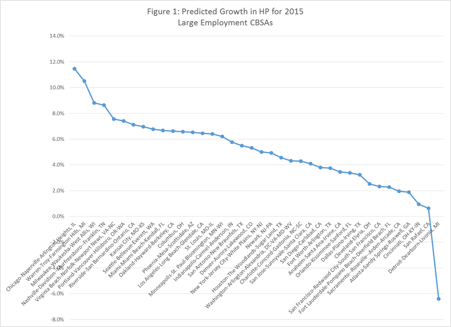
Insights about the accuracy of these estimates can be obtained by examining the standard errors of the predicted values for 2014:Q4, which is the last period of data used in the estimation. The average standard error for this group of CBSAs is 0.37 of one percent (0.37%). This error computes the error of the equations used to make the predictions. It does not include potential errors in the predicted values of variables used to compute the 2015 HP predictions such as employment, the affordable price, the national house price index, and others. However, it may offer some confidence in the predicted values for 2015. As such and conditional on the predicted values of the various exogenous variables, we feel confident in identifying a number of CBSAs in which the predicted values are substantially above or below the average predicted values. These include Chicago, Warren, Milwaukee, Nashville, and Virginia Beach at the top of the list because the predicted values for these CBSAs are at least 10 times the standard errors of their predicted values. The predictions for five of the CBSAs at the bottom of the list also fit this criterion: Fort Lauderdale; Atlanta; Cincinnati; San Rafael, and Detroit. Sacramento is also at the bottom of the list but its standard error is relatively large. Indeed, five of the CBSAs with the largest prediction errors are in California: Oakland (.75%); San Jose (.74%); San Francisco (.78%); Sacramento (.45%), and San Rafael (.45%). The other two with standard errors above 0.45 percent are Warren (.54%) and Detroit (.60%).
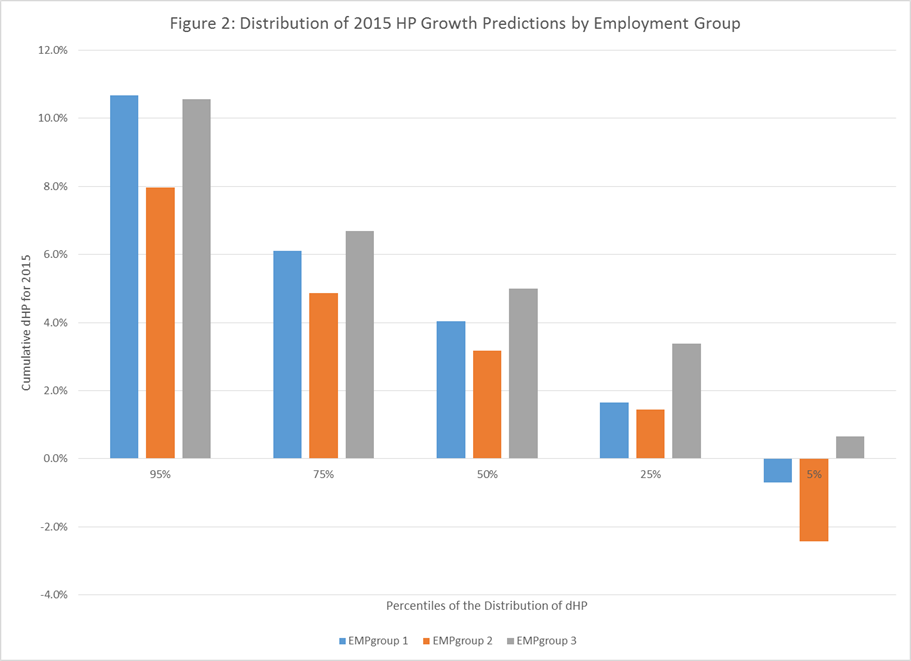
Figure 2 above, contains summary information about the 2015 predictions of cumulative house price changes for the three employment groups. The median price changes are highest for the largest employment group and smallest for the CBSAs in the mid-sized employment group (3.2 percent). One key takeaway from the figure is the wide distribution of predictions for 2015. The interquartile range (75th less 25th percentile) within each employment group is 4.4 percent for the smallest employment group, and 3.4 and 3.3 percent for the other two employment groups. We judge this to be an indicator of wide future price changes among these CBSAs.
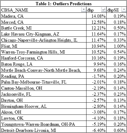
Table 1 above, focuses upon the outliers. Madera and Merced, CA are at the top of the list with predicted price changes of 14 and 13 percent, respectively. Note that the standard errors of these predictions are below average. Eight CBSAs are predicted to have price increases in excess of 10 percent. Ten others have predicted changes of less than 1.7 percent, which is the 5th percentile of the distribution. Detroit is at the bottom of the list at -6.4 percent and the Youngstown-Warren-Boardman, OH-PA CBSA is at -5.19 percent.
A Look at the Root Drivers of the Predictions
The primary causes of the variations in these final predictions among metropolitan areas are the three sets of coefficients estimates, widely varying values of the underlying factors in the model, and the predicted future values of employment and the affordable price. Even the predictions of the national US HP Index affects the distribution of the predictions among metro areas because each group of metro areas has its own “beta” or response to movements in the national house price index. Some insights about the importance of these various factors are obtained by running a simple regression of the cumulative predicted price change for 2015 for all 204 CBSAs as a function of a mixture of both LR and SR drivers. These results are contained in Table 2.
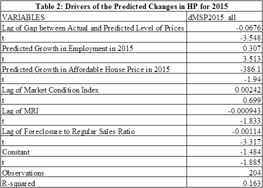
Here are a few key observations that emerge from an analysis of these predictions:
• The four period lag in the residual from the first equation (L4.MSPres_all) has a negative and statistically significant impact on the predicted price change for 2015. That is, areas in which the actual levels of the median house price at the end of 2014 were above the levels predicted by the core long-run drivers – employment and the affordable price — predicted price changes in 2015 were smaller, all else equal.
• Larger predicted growth rates in employment for 2015 have a positive impact, as expected. Larger predicted growth rates in the affordable price have a negative impact, which is unexpected. These signs likely represent substantial collinearity in these two variables.
• Two of the short-run market conditions variables have strong and expected impacts on the predictions. A larger MRI at the end of 2014 leads to smaller price forecasts. Areas with relatively larger numbers of foreclosure sales also have slower predicted growth.
Overall, these results are consistent with the importance of including measures of both LR and SR conditions in a forecast of the future.
Summary and Key Conclusions
Predicting future movements in house prices is both important and challenging. Many decisions rest upon a sense of where house prices are expected to move in the future. Housing investment decisions is the best example of what we have in mind. Also, CA’s Credit Risk Model, which measures variations in the credit risk of residential mortgage lending, depends heavily upon such predictions. See our recent article that uses the CRM to measure regional variations in credit risk.
Our approach to modelling future price changes rests heavily upon the belief that such changes are heavily dependent upon local market conditions. These include not only core drivers such as local employment and the affordable price, but also the responsiveness of local house prices to these variables. Our approach also draws upon both long-run factors and short-run market conditions to predict prices one year ahead. The key long-run factor is the gap between the level of prices and the level predicted by the levels of employment and the affordable price. All else equal, the larger this gap, the slower is the predicted growth in prices. The three short-run factors in our model are the months of remaining inventory in the amount of listings, an index of a variety of market conditions, and, especially, the ratio of total sales represented by foreclosure sales.
Download a PDF file of this research paper here.