by Dr. Michael Sklarz and Dr. Norman Miller | August 1, 2016
Introduction
It is becoming common when ordering appraisals on new loans or refi applications to also include an AVM (automated valuation model) as these are relatively inexpensive ways to quickly audit value estimates. A previous study found that the loan to value may be understated, since over 92% of all appraisals at the time of initial loan application match or exceed the purchase price on new contracts.[1] Aside from concerns over bias in valuation, uncertainty should be another concern. Value error can be estimated and is provided with AVMs but is conspicuously absent from traditional appraisals. This estimate of the uncertainty behind the value estimate is a critical component of risk analysis not yet being utilized in the market.
Property values are uncertain for a variety of reasons including but not limited to heterogeneity of the neighborhood making comparison difficult, rapidly changing prices or market conditions, or atypical property not in conformance with the neighborhood. Here we demonstrate a unique way to use such information, by adjusting the LTV towards an estimate of value not based the most probable average price but one that takes into account a higher than average proportion of the distribution of possible values. In other words, we can answer the question with various levels of confidence: how low could the market value be?
Statistically, market values are derived to seek the most probable price as of a given date. But the dispersion of prices varies significantly by neighborhood. Below in Exhibit 1, we provide two examples of such price dispersion. Neighborhood A is characterized by a large degree of price dispersion from having multiple developments occur over many years, while neighborhood B is characterized by a neighborhood built out by one developer over two years.
Exhibit 1: Price Dispersion Varies by Neighborhood
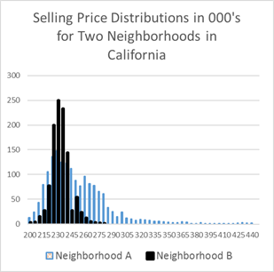
In both neighborhoods above the most probable price for the average home would be the similar whether the uncertainty behind the value estimate was low or high. But, if we choose to use any confidence level above 50%, this takes into account the uncertainty reflected by the price dispersion. AVMs provide a forecast standard deviation that can be used for exactly this purpose. The standard deviation of the estimate is related to the frequency and quality (degree of similarity) of information available at the time on comparable property. Here we are proposing that lenders or mortgage investors might simply request, not just the most probable price, but also the value estimate based on a given one tailed confidence level. One tail is all that is required since mortgage lenders do not care if a property is worth more than the estimate, but they do care if it is worth less.
Here we assume a normal distribution and show how many standard deviations we must add to the mean or subtract in order to be confident about the value estimate.
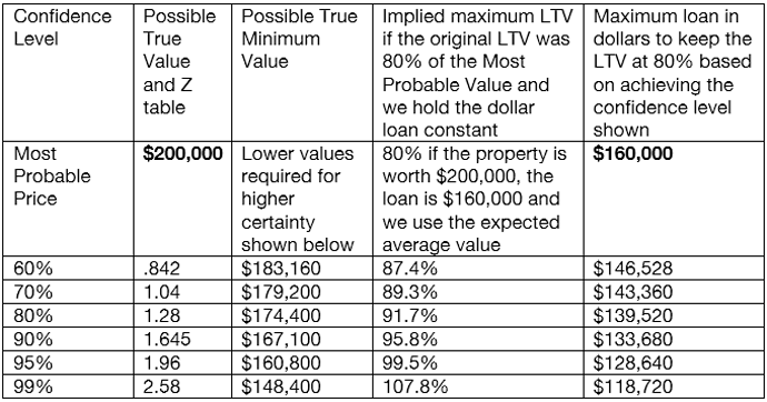
Exhibit 2: Standard Deviations Required to Derive a Minimum Value Estimate

Next, let’s apply these parameters to a given property and see how the LTV would change based on the proportion of certainty we require behind the value. For a given property the standard deviation of the estimate of value is 10%. Then the following implications are derivable with this simple additional piece of information about value:
Exhibit 3: How the loan must change to account for value uncertainty.
Reality Check
Very few lenders will need to go to the 99% confidence level even for conservative portfolio loans. But just going to the 60% confidence level or even 55%, a z score of .7554, would be one way to take into account the uncertainty behind values. Neighborhoods where values are easy to estimate will have low standard deviations, perhaps as low as 5%, and no adjustment in the dollar value of the loan may be warranted. This point is expanded below in Exhibit 5. But when values are uncertain, whether because the neighborhood is at a turning point in the market or because properties in the neighborhood are simply very hard to compare and appraise with high degrees of accuracy, then an adjusted LTV or adjusted dollar loan seem to be prudent risk management strategies.
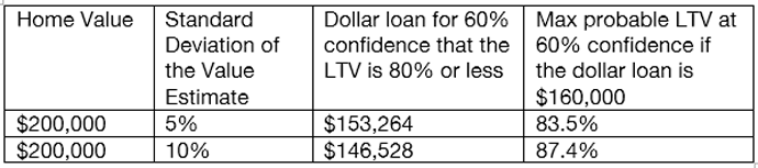
Another way to look at the benefits of using value uncertainty would be to determine dollar loans that are equal in LTV-risk for various neighborhoods. Using a 60% confidence level, and comparing two similar priced neighborhoods but with different standard deviations we would get the following result, starting with an assumed base case of an 80% LTV or $160,000.
Exhibit 4: Range of True LTV with Uncertainty
Accounting for Market Conditions
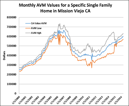
Not only are some properties and some neighborhoods more difficult to value with a pinpoint estimate based on heterogeneity, market conditions vary over time and this will also increase/decrease value certainty. When market trading is thin, when prices are moving quickly in either direction or at turning points we can observe much less certainty in pinpoint value estimates. In Exhibit 5 below we show the most probable value, the low and the high value with a similar confidence range across time. Note how in the years 2000 through 2005 the range of value estimates for the same home are fairly tight. Then after trading thinned and prices fell, the uncertainty increased dramatically. By considering price dispersion via a simple standard deviation of the estimate we can account for such uncertainty in a prudent risk management way.
Exhibit 5: Value Range for the Same Confidence Level Over Time
Conclusion: Equal LTVs are NOT Equal Risk
What we have learned from the last housing downturn is that standardized LTV based lending without regard to the certainty behind the values allows a false sense of security. The reality is that a 90% LTV in a homogeneous and stable neighborhood may be lower risk than an 80% LTV in an area of high price volatility and or uncertainty. The use of standard LTVs while ignoring the risk related information available on value estimates seems imprudent and irresponsible. It is not difficult to incorporate a modest increase in the confidence level from the 50% expected most probable value now provided by appraisals to something just a touch higher. Even moving to 60% confidence would greatly enhance risk analysis and allow for more prudent risk management.
Certainly a forecast of future values would be even more valuable and when prices are expected to decline, initial LTVs should be adjusted downward.[2] We can forecast values three years out with some reasonable level of accuracy, but there will be third party vendors that provide more optimistic forecasts than others and such a system would be subject to gaming. Utilizing uncertainty in current value estimates is not speculative and yet still provides a significantly better way to handle LTV based risk.
References
Agarwal, Sumit, Brent Ambrose and Vincent Yao, “The Limits of Regulation: Appraisal Bias in the Mortgage Market”, The Social Science Research Network, December, 2011.
Calem, Paul S., Lauren Lambie-Hanson and Leonard I. Nakamura, “Information Losses in Home Purhcase Appraisals”, Federal Reserve Bank of Philadelphia (Working Paper No. 15-11), March, 2015.
Griffin, John M. and Gonzola Maturana, “Did Dubious Mortgage Origination Practices Distort House Prices?”, The Review of Financial Studies, January, 2016.
Miller, Norm G. and Michael Sklarz, Integrating Real Estate Market Conditions into Home Price Forecast Systems” Journal of Housing Research, 21:2, 2012.
Download a PDF file of this research paper here.
[1] For an example of home price forecasting see “Integrating Market Conditions into Home Price Forecasting Systems” by Miller and Sklarz, 2012.
[2] This is from the work of Calem et al, 2015, for 2007-2012, During the 2005-2007 period the appraisals matched or exceed even a higher percentage of purchase prices. See Griffin and Maturana, 2016.