by Dr. Michael Sklarz* and Dr. Norman Miller** | February 12, 2019
Download a PDF file of this research paper here.
Abstract
For decades most housing economist have used median home prices and median household incomes along with current mortgage rates and entry level loan-to-value ratios, to generate a housing affordability index. Such an index does little to determine how affordable housing really is for the existing population. It does provide a relevant index for the trends in affordability and nothing more. In an era where housing crises are presumed to be ubiquitous, we should take a deeper look at how anyone can afford to live in expensive cities. Here we take a look at one of those expensive cities to illustrate why a deeper dive on affordability is required.
Introduction
In 2017 we wrote a paper entitled “The Story of Entry Level Housing Affordability in the USA Considering Price Tiers and Property Taxes”. In that paper we tried to convince housing analysts, and the media they cater to, that instead of using median home prices and income, we should use something more reflective of starter homes and we should also consider property taxes as a significant cost for buyers in some markets. While we have not given up on the need for better indices, here we focus on just one market, San Diego County, California, to illustrate a few of the biases in how we judge affordability. These include the fact that most existing residents faced a different set of prices when they purchased, and that the use of medians or means of current sales transactions are very much influenced by a high end of extremely expensive homes which may not be typical in some markets. We also note that the actual distribution of home values may differ significantly from those reflected in current sales prices. When current sales prices are used for affordability calculations and policy related conclusions, rather than the values reflective of an entire market, the reality behind affordability is distorted. One last relevant factor in California is that Proposition 13 which limits increases in property taxes to no more than 2% per year, also increases home tenures, decreases housing supply and artificially increases home prices on those homes which do sell.[1] This is not to say there is not a real housing affordability gap in the market and we acknowledge that homelessness is caused, in part, by high housing costs. But the portrayal that hardly anyone can afford housing, even in markets like San Diego is not true.
Below in Exhibit 1 we see the average prices in San Diego County for single family homes from the year 2000 through the year 2018. The median single-family sales price for 2018 was $618,000 with an average or mean well above that. The median is the figure which sits in the center of a distribution with half the transactions on the right and half on the left. The mean of well over $700,000 is based on the simple average of all transactions and is very much influenced by the higher priced tail we see in Exhibit 2 below. The mode, or most frequent sales price is well below the mean.
Exhibit 1: The Big Picture on Prices in San Diego
County by Quarters Through 2018
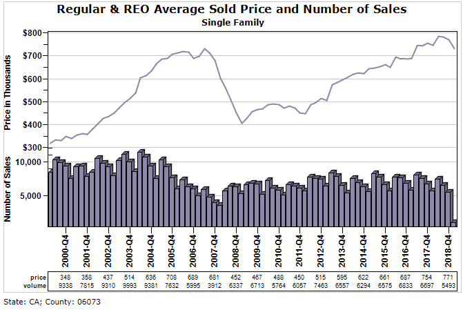
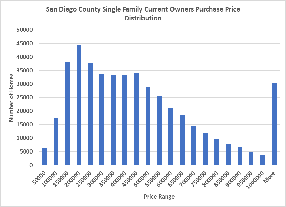
One might expect that the average transaction price shown in Exhibit 1 is typical for buyers in this market, but it is not. In Exhibit 2 we show the prices that 2018 residents actually paid for their homes regardless of when they bought. Some owners bought a few years ago and some bought twenty or more years ago. All of these prices are included in Exhibit 2. In Exhibit 2 below we see the mode or most frequent transaction price for current owners is closer to $200,000, while the mean or average price paid is $476,000 so how can the mode be so low and the average be approximately 238 percent of the mode? The answer lies in the tail. There are a modest number of very expensive homes sold each year in San Diego, but they are expensive enough to impact the average price. So, if you would use the 2018 median income of the county of $70,588 per household this would support a home price of $342,000 based on a 30-year mortgage loan and loan to value ratio of 80% with a 5% rate and monthly payments of roughly $1470 using 25% of the annual income. This is far below the average transaction price reported of $771,000 in 2018 and it would be easy to sensationalize how unaffordable average home prices are in San Diego County, CA. But if we use the distribution of actual transaction prices paid, as shown in Exhibit 2, we could have concluded that the average household in San Diego can afford over half of the homes actually purchased in 2018, and they can afford the prices they actually paid if we consider that now they have much more equity in these homes and would not need to borrow 80% of the purchase price, as assumed by affordability analysts. Existing owners may gripe about affordability but they are also the beneficiaries of these high home prices and many are house rich as a result. If they do buy a new home, they will typically use a much lower mortgage as a percentage of the next home than they did on their first home. This equity is ignored in typical housing affordability indices, which are much more appropriate for first time home buyers.
Exhibit 2: Distribution of Sales Prices for Current
Owners of Single-Family Homes in San Diego County
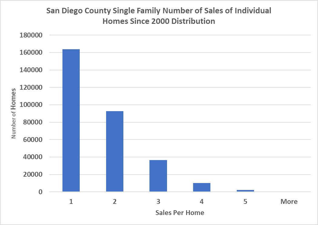
There is another bias on the use of average transaction prices, for judging affordability. The transaction prices are reflective of the turnover in the market and some homes turn over more frequently, at prices incongruent with underlying values. In Exhibit 3 we observe that there are some homes which sell as many as four or five times in a period of only 18 years and each sale becomes part of the calculation for average prices, but these transactions, like the high-end tail sales may not be reflective of the more typical home that sells only once in 18 years. Again, the mode is far from the mean for this statistic on turnover.
Exhibit 3: How many times homes are sold since the
year 2000?
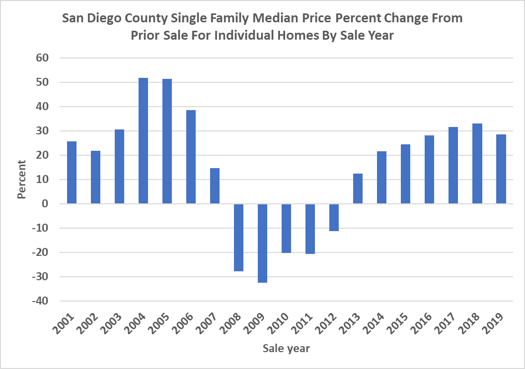
In Exhibit 4 below we show the median home price percent change from the prior sale over time. In 2005 and 2006 we observe many sellers capitalizing on the large increase in prices since 2000 through 2006 and cashing out near the peak. Those who got into the cycle too late and needed to sell, did so at losses as reflected in 2009 through 2012. Those who could ride out the cycle held on, waiting for positive appreciation and selling at modest annual gains in the later years. The point here is that median and average homes prices are reflective of turnover in a given year and this turnover is influenced by the equity value trends. Sales volumes in 2004 and 2005 were much higher than in 2008 because most owners had significant equity if they sold at prices approaching a price peak. Those selling in 2008 made no profit on average, but sold because they had to. The patient owners who sat out the peak and the trough were not reflected in these median figures. If we used average market value of the entire stock of housing the fluctuations in any current value index would be much lower. Perhaps that is what we should use to judge affordability?
Exhibit 4: High Variance in Median Home Prices
from Prior Sale
Conclusions
Housing affordability measurements based on only median home prices and median household incomes are probably antiquated. Today, with richer data sets we can utilize more of the relevant information including segmenting the market into price tiers or valuing all the homes in each market. We should also not rely upon averages in markets where extreme price variances exist. Rather we should examine a distribution of prices in order to understand what is truly typical in a given market. Housing affordability may be a crisis for some renters who would like to enter the owner segment of the market. But many of the existing owners have benefitted from these high prices and would use this equity in the next purchase, if they do decide to sell. They also may decide to buy a typical home, not an average home and that will be at a much lower price than those reported as averages.
*Collateral Analytics CEO
**University of San Diego School of Business and Collateral Analytics Research
Footnotes
[1] See “A Note on the Impact of Prop 13 on Effective Tax Rates, Turnover, and Home Prices”. Journal of Housing Research: 2016, Vol. 25, No. 2, pp. 213-223.