Download a PDF file of this research paper here.
Introduction
Collateral Analytics has created a new set of Daily Home Price Indexes, HPIs, for single-family residential transactions in a number of major metros.[1] Residential real estate has always been a very important asset class for the typical household since a high percentage of each household’s net worth is attributed to it. It is well known that daily and, even, intraday price data is available for many years for stocks, commodities, currencies, bonds, and cryptocurrencies for many years. Our motivation is to provide some of this same high frequency market information for home prices to the real estate market. Hopefully, more frequent information will lead to better informed decisions and result in more informationally efficient housing markets.
There are also other uses for such timely information beyond home buyers and sellers. Efficient data can help inform those involved in home building, real estate brokerage, appraisals, mortgage lending and mortgage insurance to name a few interested parties. At the same time, there has been an institutionalization of single-family housing in recent years including a number of single-family rental REITs. [2] All of these players in the housing industry should be interested in as timely an information flow as possible on home prices. The new Daily HPIs will be an important improvement over the current home price series which are reported monthly or quarterly and with a significant lag.
Our initial set of single family HPIs cover the same 20 markets as the Case Shiller, C-S, Home Price Indexes. In addition to highlighting these widely followed markets, we thought that this would be a good way to show how the Daily HPIs compare with the C-S monthly ones. We do this comparison in our next article.
The first thing that we noticed when creating the Daily HPIs is that the actual data is quite volatile. There are a number of reasons for this including the fact that there is a different mix of single-family homes selling each day with regard to home size, age, quality, and features. To help normalize this, we use the sold price per square foot of living area as the HPI metric and then do simple smoothing (prior seven days) to these values to reduce the inherent volatility.
Aside from some normal seasonality, we observe that housing exhibits volatility much like the stock market. At any point in time, there is a range of prices over which real estate can trade. Below, we review some valuation terminology, along with fundamentals driving observed prices, followed by a sample of graphs that compare real estate to stocks.
Value and Price Concepts
Value concepts are always theoretical in nature, while price is factual in nature. There can be a specific “asking price” or “list price” and “selling price”, about which there should be no dispute or range of opinion. But, value is, by nature, an opinion and in the absence of a perfectly competitive market, there can be no certainty that the value sought is resolutely true or unchallengeable. An appraisal is based upon a defined value and when seeking “fair market value”, defined below, is statistically based upon the most probable price.
Fair Market Value: The highest price a willing buyer would pay and a willing seller would accept, both fully informed and without duress or unusual financing. There are many other definitions of market value but all contain normative and typical descriptors about the transaction described. When appraisers use the most probable price to estimate the market value they seek transactions from informed buyers and sellers acting without undue pressures or circumstances. The term fair market value is generally based on definitions from the Appraisal Institute, and while similar to the above definition, ignores the fact that market value is really a realistic range of possible prices, and not a single point. The more unique the property or thinner the market, the larger is this range for any given property.
In economics we use the term “reservation price” to depict the maximum price a buyer would pay or minimum price a seller would accept for a property of interest. A reservation price is akin to an investment value and is unique to a given buyer or seller. Reservation prices can differ between buyers and sellers, based on differences in tastes and preferences, risk perceptions, wealth, access to capital, tax circumstances and for other reasons.
Time Targeted Value: A term trade marked by Collateral Analytics that produces an estimate of realistic prices for quicker than normal sales.[3] For example, if the normal marketing days on market is 120 and a seller wants to know the value of their property with a 30 to 60 day sale, a discount will be calculated based on an algorithm that considers how much discounts speed up market interest and offers. Market conditions and price tiers must be considered in these calculations and slower or distressed markets require much larger discounts to sell quickly, akin to an auction or liquidation price estimate. Fair market value assumes normal or typical marketing time while time targeted pricing adjusts the price to match the desired time to sell.
Equilibrium or intrinsic value: Another definition of value which appraisers are occasionally called upon to wrestle with is what is sometimes called “equilibrium value”. “Market value” normally represents an equilibrium value. However, real estate markets may not be perfectly “efficient” in the sense that market values may not always fully and immediately reflect all the publicly available information relevant to property values. In such circumstances, property market values may experience persistent movements or “swings” in one direction or another, above and below the long run equilibrium value. If the appraiser feels the current prices are temporary, then they may estimate an adjusted price which they consider to be supportable in the longer run. This supportable value may also be called intrinsic value, based on longer term fundamentals.
What drives real estate prices?
What a buyer will pay and a seller will accept at any point in time is actually a range of reservation prices. If these distributions for buyers and sellers overlap, then it is possible to consummate a transaction price agreeable to both. When tastes vary substantially or when interest rates are changing and there is uncertainty in the economy, we will see a larger range of selling prices for similar and competing property. Likewise, when a property has unique features, unique views or is unusual in some respect, this makes it more difficult to compare it to other properties, thus, the range of possible market prices will be larger.
Information and search are essential and significant features of the housing market, where buyers are looking at substitute properties and sellers are looking for potential buyers. Some buyers have higher search costs than others and this may determine how much information they collect prior to putting in an offer on a home of interest. Sellers, also have different levels of urgency within which they must sell and this affects the prices they are willing to accept. Some luck enters the picture on both sides for buyers and sellers in finding each other.
What makes it even harder to determine value is that the market does not stand still. Mortgage rates change over time, the number of similar homes for sale may change, businesses expand and close within a given region and all these dynamic factors create a dynamic real estate market which may produce a range of prices for a given property.
For any given property on the market for sale, on any given date, there will be a range of possible selling prices not a single point, even though appraisers are most often asked to provide a single point estimate ignoring the potential price dispersion that underlies such estimates. Automated valuation models, AVMs, typically provide information on the range of likely prices when estimating value. These range estimates provide useful information for mortgage risk metrics, yet, the price dispersion estimates are not yet being utilized by most lenders. Here, we also provide some useful metrics, that we hope the market will eventually consider. Below, we provide some results using a new price index based on selling prices per square foot of living area and compare these to stock price movements.
Why a new home price index?
There are several reasons why a new residential price index will be of interest to the market. First, by using a simpler index we can produce it with very little delay, almost in real time. Second, this index includes the entire resale market even when no prior sale is available. It can be argued that such an index is more reflective of the market as a whole and it will be based on a slightly younger set of properties than repeat sales methodologies. Third, this index is available for a large number of metropolitan markets and will be available for various submarkets and cities over time.
Among the most followed indices today for residential property are:
1. S&P Case-Shiller, now produced by Core Logic, developed by Karl Case, PhD and Robert Shiller, PhD and calculated for 1987 onward for both the nation, and several composites including 10 or 20 metros. Case-Shiller is a repeat sale index requiring a sample of at least two sales for price trend calculations. It is published monthly. This use of repeat sales eliminates the need for quality adjustments although there will be variation in real depreciation and capital improvements that distort results. Case-Shiller also filters out sale under 12 months but retains some bank REO sales, if transfers occur after 12 months, and these distressed sales can at time alter the general trend. When prices fell in 2008-2010 the Case-Shiller index tended to overstate the true market decline, as the proportion of distressed sales affected the index. When prices later increased, the Case-Shiller index tended to overstate the increase as the starting base was lower during the trough of the housing crisis. While Case-Shiller is generally a reliable index for existing home markets, it is produced with a significant lag to the market, typically around two months and a few days.
2. The National Association of REALTORs (NAR) median home price index is published by metro and for the US as a whole. It is a reasonable proxy for homes that do sell, but the mix of homes by size and quality many vary affecting the index.
3. The Federal Housing Finance Agency (FHFA) publishes a quality adjusted home price index that uses a hedonic model to control for size, feature and quality differences. This home price index (HPI) is published monthly with a lag and is considered a more accurate indication of typical home price trends. The FHFA index only includes homes that are financed by conforming home limits which change over time but do not include the upper price tiers. These limits vary by market but right now are typically about $510,000.
A New Simple Real Time Index
While the above indices are all useful, producing a more current price index is possible, albeit with some simplification. Here we propose a simple index that controls for size by running the index in price per square foot. We also control for age by pairing the sample of all possible transactions down just enough such that the average age of the homes, from the first calculation of the index increases by exactly one month for each month the index is produced. We also include a modest number of new homes, if they are sold through the multiple listing service, they are not part of the repeat sales index. Thus, this index is not necessarily going to be identical to the S&P Case Shiller Indices. While we can produce these price per square foot statistics daily, in the chart below we used the 15th of the month.
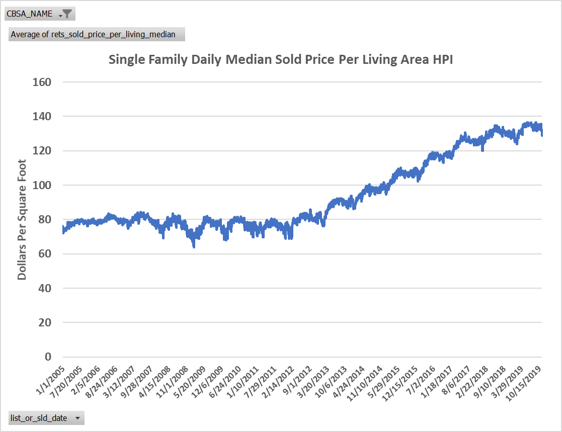
Below we show Los Angeles and Dallas market graphs (Exhibits 1A and 1B and 2A and 2B) where we compare in 1A and 2A the median home sold prices to the 1B and 2B median sold prices per square foot. Note how the simple adjustment for size significantly reduces the dispersion of prices.
Exhibit 1A: Los Angeles Daily Median Home Prices 2005-2019

Exhibit 1B: Los Angeles Daily Median Home Prices Per Square Foot of Living Area 2005-2019
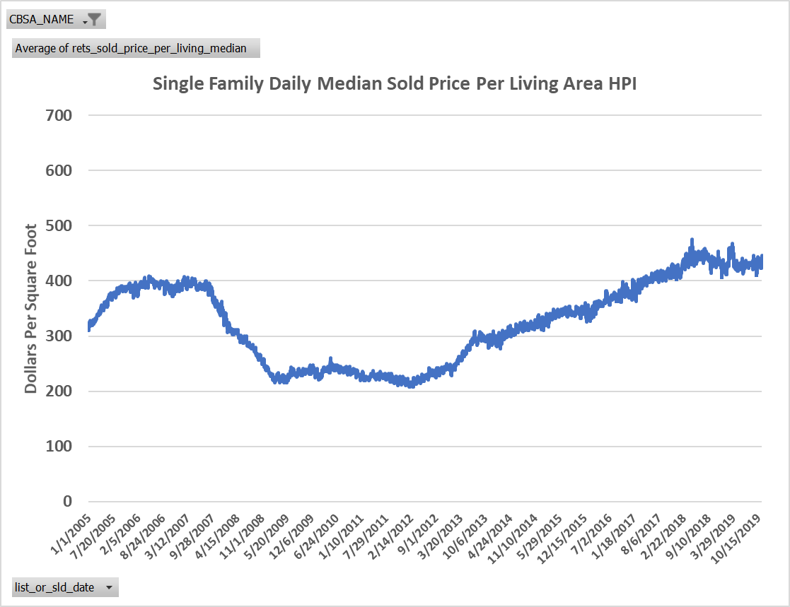
Exhibit 2A: Dallas Daily Median Home Prices 2005-2019
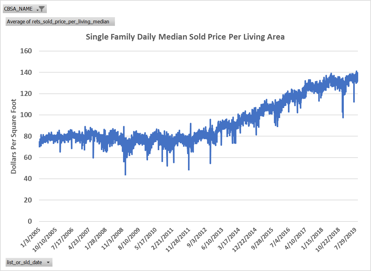
Exhibit 2B: Dallas Daily Median Home Prices Per Square Foot of Living Area 2005-2019
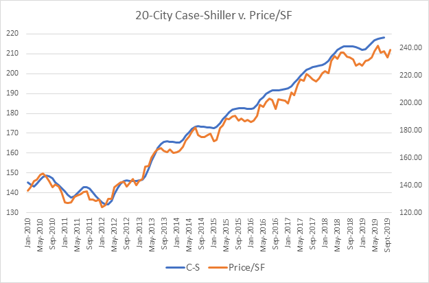
How does the simple HPI compare to Case Shiller? Exhibit 3 below shows the S&P Case Shiller Index for the US based on 20 markets compared to our HPI based on price per square foot of living area for the same markets. This repeat sales index appears to have slightly less seasonal amplitude but is remarkably correlated, at 99.61%, with the price per square foot averaged for all the same markets.
Exhibit 3: Case Shiller’s 20 Market Index versus Price Per Square Foot for the Same 20 Markets
How does the Collateral Analytics HPI Compare to Stocks?
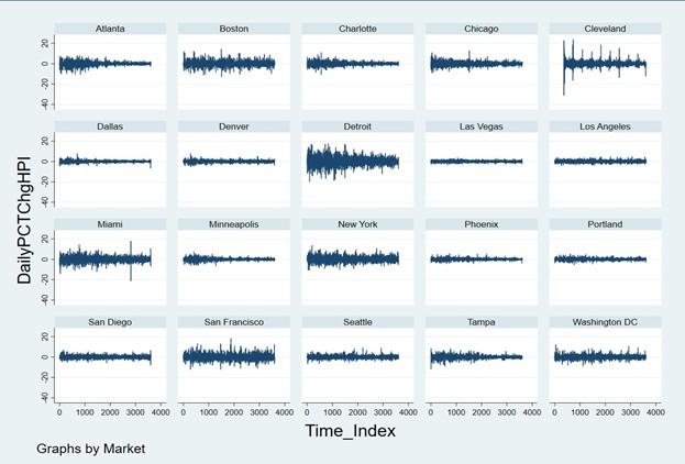
Daily price movements within the 20 markets tracked by Case Shiller were selected for comparison in Exhibit 4 below. We observe some markets trade with more noise and volatility than others as seen in the Daily Volatility charts in Exhibit 5. While these graphs are merely for illustrative purposes, we have a table below that calculates actual percentage changes on a daily basis using changes in the average and changes in the median.
Exhibit 4: Twenty CBSA Daily Home Price Per Square Foot Trends 2010 to 2019
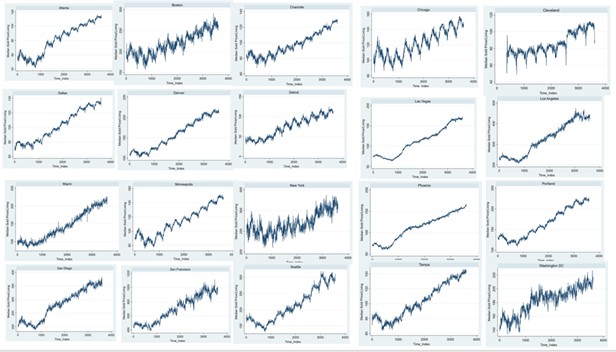
Exhibit 5: Twenty CBSA Daily Home Price Per Square Foot Volatility 2010 to 2019
The daily percentage changes for the CBSAs graphed above are calculated in the following table in Exhibit 6. The first column is the change in the average price per square foot and the second column is the change in the median price per square foot, expressed in decimal form where 1.0 would be 1%. Using the average change in the average price per square foot results in something close to a 1 percent change per day. Using the change in the median prices results in something closer to .6% per day.
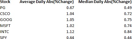
Exhibit 6: Price Per Square Foot Volatility Calculations for CBSAs and Selected Stocks

By comparison, the average change in the averages and median prices of trades, for well- established public companies is shown below.
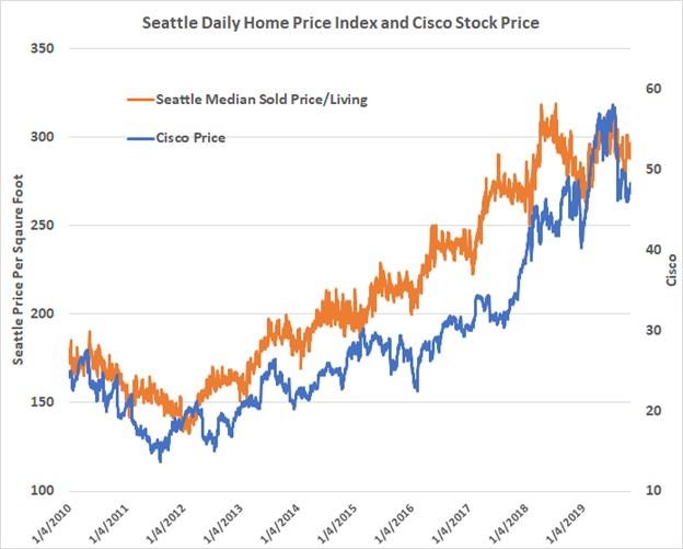
One of these CBSAs, Seattle is compared to Cisco stock over the period from the start of 2010 to November of 2019. While the residential price volatility is slightly higher, it does include more noise from different quality property in the daily mix.
Exhibit 7: Seattle Homes Prices versus Cisco Stock Prices
Price Change Calculations Illustrated
For Seattle, we have the following price change statistics calculated for November 6, 2019: Daily price change = -2.305%
1 Month = +1.502%
1 Year = +2.163%
5 Years = +52.909%
Clearly the shorter time spans are less reliable by themselves but with repeated calculations we can observe a trend.
Conclusions
Here we provide a discussion of how real estate values are defined, how values are estimated via prices, and the various types of indices currently available to the public. A new daily index based on prices per square foot of living area is produced here and will be reported in the future for a number of metro markets. These indices will, hopefully, be utilized by market analysts in a variety of ways. For example, we can estimate the C-S index well in advance. We can forecast with less lagged information which way prices are heading and if we are approaching a turning point in the market. Real estate is far too valuable an asset not to have the same type of information available that is present for the financial markets and here we embark on a mission to expand the available data for all market participants and supporting professionals.
Footnotes
[1] The starting set is the same as used for Case Shiller indices but this will be expanded rather quickly for most
[2] See https://www.reit.com/news/reit-magazine/may-june-2017/reits-flourishing-single-family-home-rental-segment
[3] Term coined and used since 2007 and includes time targeted pricing as well as time targeted
[4] See https://www.fhfa.gov/DataTools/Downloads/Pages/Conforming-Loan-Limits.aspx