Is A New Home Price Bubble Forming?

by Michael Sklarz, Ph.D., Jim Follain Ph.D., and Norm Miller Ph.D.

INTRODUCTION

There has been growing speculation among some economists and real estate market observers that there is another bubble forming in the U.S. housing market or in various metropolitan areas. Our analysis based on a number of approaches we have used over the years to identify home price bubbles is that we are far from bubble territory on a national or metropolitan level and that anyone claiming otherwise is looking to sensationalize an issue which does not exist.  However, there are some smaller cities and/or ZIP Codes which are exhibiting frothy behavior and which will be discussed.

When discussing “price bubbles”, we feel that there are few terms which are more widely used and less understood. One definition is that a bubble is an unsustainable price trend fueled by speculation that prices will continue to increase. In theory, the price of an asset in market equilibrium should be a reflection of its intrinsic value. In the case of stocks, one typically looks at earnings and dividends as the basis for intrinsic value. With home prices, there are several ways to look at intrinsic value. One is the current and future “imputed rents” the owner is paying himself to live in his residence. A second is the so- called “affordable price”, i.e. the price that the typical household can afford based on local income, wealth and current mortgage rates. Of these, mortgage rates are usually the most volatile and a rapid increase in mortgage rates will generally dampen real estate prices. In markets where wealth is volatile, say for markets with a heavy concentration of recently successful tech start-ups, changes in the value of these companies could also be considered a volatile factor driving prices. Changes in incomes, on the other hand, rarely change rapidly and are less likely to trigger rapid price declines except in markets with little industrial diversification.

The difficulty in understanding asset prices is that there is always an element of expectations built into them. In the case of home prices, these expectations might take the form of higher future rents, higher household incomes or wealth, or lower mortgage rates. This can create a disconnection between the home’s current intrinsic value and market values based on longer term expectations. A bubble occurs when prices keep rising only because they are expected to keep rising, rather than being based on the fundamentals of income, wealth, and debt costs.

As opposed to stocks and commodities, there are a number of factors, which should reduce the likelihood of home price bubbles. One is the fact that the typical home buyer takes out a mortgage and often these mortgages are fixed rate instruments. Second, the buyer must be able to financially qualify for the purchase. This should set a constraint of how high the price to income levels can reach in a local market, especially since most people use significant debt when purchasing a home. Another possible constraint is that a mortgage lender will require an appraisal on the home which means that there is a second and, hopefully, objective opinion of its true value.[1]

Another reason why we do not use the term “price bubble” freely is that real ones are very infrequent. Examples of real bubbles include, stock prices in 1929, 1987, and NASDAQ stocks in 2000, gold and silver in 1980, Japanese land and real estate prices in 1989-90, and, of course, home prices in the U.S. in 2005-2007. Based on these rare examples, it is reasonable to say that true bubbles only occur on average once in a generation.

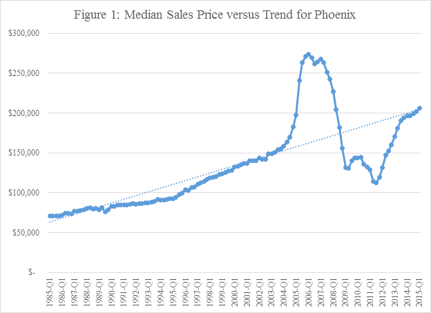
The intuitive notion of a bubble can be seen in the Figure 1 chart below. Here we see the Phoenix CBSA median single family price along with a trend line running from 1985 to current. Viewed this way, the appreciation rates in the 2005-2006 period were clearly an example of prices getting ahead of any kind of sustainable trend. This led to a severe decline or correction to the longer-term trend before the market found a bottom in 2009-2011. Note that prices are now moving back to their longer term trend level and note that often when prices collapse they overshoot fundamental values on the downside as well.

INDICATORS SUGGESTED BY THE COLLATERAL ANALYTICS HP MODEL

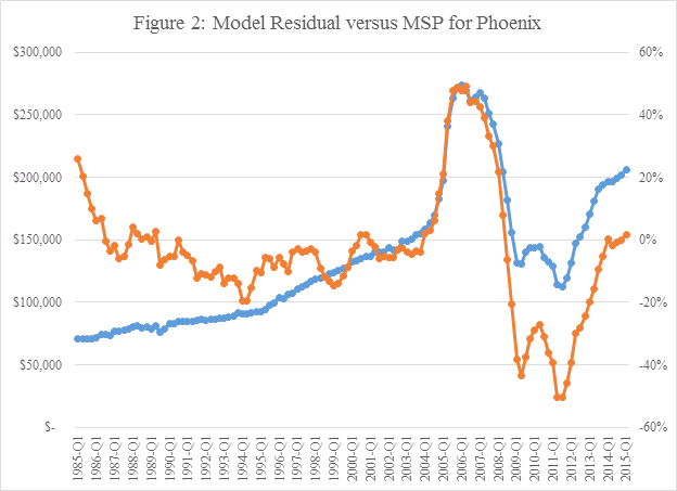
The Collateral Analytics Home Price Forecast Models use a number of fundamental and technical drivers (independent variables) which can provide a more economically based way to analyze home price intrinsic value and, thus, overvaluation (or undervaluation). Figure 2 below shows the Phoenix median price and the residual expressed as a percentage difference between the Median Sale Price (MSP) and the model prediction of MSP. This residual provides an excellent way to identify home price bubbles. As seen in Figure 2, the residual during the 2005-2006 period was extraordinary.

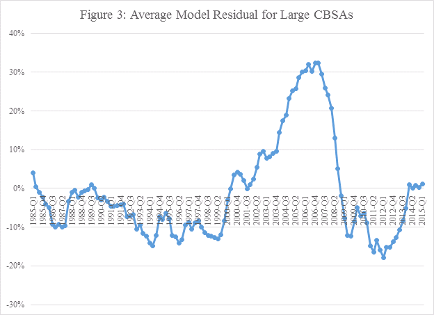
We have created home price models for nearly 400 CBSAs around the U.S., which include many of the areas that were widely acknowledged to having had price bubbles in the 2005-2006 period and which exhibited similar patterns with regard to the residuals. Insights about the market at the end of 2015:q1 versus the historical record since the early 1980s is captured in Figure 3 below. This plots the average residual among 48 or the largest CBSAs over time. Note the sharp peak during the 2005-2006 period and the height of the bubble. On average, the average residual is about equal to zero over this entire time period.

There are, however, some potential exceptions that may be showing potential signs of a bubble. These are highlighted in Table 1. Column 3 shows the average annualized value of residuals for 35 large CBSAs estimated with the model using data through 2015:q1. These are ranked from the lowest to the largest residuals. The second column shows the size of the residuals for 2006:q1 using the same model. The last column shows the difference in the sizes of the residuals in 2005 and 2014 using the current model (column 3 less column 2).

First, the average residual as of 2015:q1 for this group of CBSAs is 3 percent, but there is wide variation around it. The smallest is -47 percent for Detroit and the largest is +29 percent for San Rafael. Clearly, all markets are not the same. Second, the average difference between the residuals in 2006:q1 and 2015:q1 is -29 percent and is lower in 2015:q1 than in 2006:q1 for 32 of these 35 CBSAs. Third, the residuals in 2015:q1 are substantial – greater than 20 percent — for 7 CBSAs; these are highlighted in red. Though substantial, these are all lower than the residuals for 2006. These include three from the SF Bay Area: Oakland, San Francisco, and San Rafael. Another SF Bay Area CBSA – San Jose – has a residual of 19 percent.

WHAT IS DRIVING THE LARGE RESIDUALS IN AT AT THE CURRENT TIME?

A key question is whether the large residuals, especially for those in the SF Bay Area, can be explained by fundamental economic forces not captured by the model or do they show signs of a bubble driven by irrational expectations about the future and, if so, highlight the possibility of a sharp drop in prices in the near future. We offer some considerations to help address this question.

Potential explanations for the relatively large residuals. Four come to mind.

-First, the areas of the San Francisco Bay Area have benefited greatly in recent years from increased wealth to those associated with the booming IT firms in the area such as Apple, Oracle, and Facebook. Perhaps the increases in wealth among many of the residents of these areas are much larger than is captured by our affordable price variable, which is driven by median household income. If so, then the potential of a bust in the housing market will be affected by future trends in the value of the wealth associated with this industry.

-Second, perhaps the demand for housing and other kinds of real estate in these areas is positively affected by international demand for real estate in the SF Bay Area. If so, then the potential risk may stem from changes in the value of the dollar and the strength of foreign economies. A sharp rise in the dollar, all else equal, would likely reduce such demand and bring about declines in housing prices.

-Third, the supply elasticity of housing in these coastal areas is likely much smaller than in most parts of the country. In such a situation, a given increase in demand by, say, 10 percent, will, all else equal, increase house prices by more than would be expected in a market with higher and a more normal supply elasticity. Again, a given drop in demand in such an environment will reduce house prices more sharply than in a more normal market.

-Fourth, the market has become dependent upon an environment with historically low interest rates. If these rates are not sustainable and policy makers begin the process of raising rates to more normal levels, then demand and house price may suffer.

Of course, the other option is that the residuals in these places capture the kind of irrational exuberance associated with the last bubble and bust.

 

A LOOK AT PRICE TO RENT RATIOS

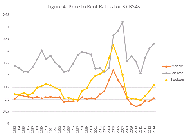
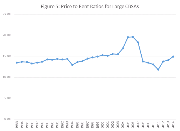
As discussed above, there are a number of other metrics which have been used to identify home price bubbles.   One is the ratio of median home price to annual rent. This is analogous to the Price-To-Earnings Ratio used to evaluate stocks and makes economic sense since the value of a property should be related to the amount of rental income (actual or imputed) which it can produce.  Figure 4 below shows the Price-To-Rent Ratio for three CBSAs – Phoenix, San Jose, and Stockton – over the same time frames as Figures 1 and 2.[2]  As seen, these ratios shoot far above historical averages during the bubble of 2006-2007.  Also, note how the current value of this indicator is very close to its longer-term average and, thus, nowhere near bubble territory.  Indeed, a plot of this ratio for 22 large CBSAs makes this point as well (See Figure 5).

 

A MORE GEOGRAPHICALLY GRANULAR REVIEW OF PRICE MOVEMENTS

Our focus at Collateral Analytics is to track the real estate market on as granular a level as possible and, in this regard, we have identified and monitor approximately 400,000 neighborhoods around the U.S. along with approximately 20,000 surrounding ZIP Codes. Of note is that there are several ZIP Codes where prices are exhibiting bubble-like characteristics. Most are in the Silicon Valley area and include markets in Palo Alto and Mountain View as seen in Figures 6 and 7 below plot the movements for single family prices for these two areas.

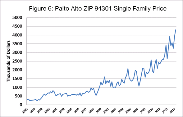
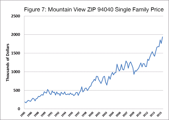
These long-term ZIP Code level charts are quite remarkable for several reasons. First, note how well prices held up during the nationwide crash in home prices in the 2008-2011 time period; second, the prices in both markets have been exhibiting exponential growth characteristics in the past several years which is one of the mathematical ways to describe bubbles.

SOME POTENTIAL IMPLICATIONS

Bubbles in the classic sense of paying more, because others are expected to continue such behavior, are rare. Indeed, our analysis indicates that there is little reason to expect a general US housing bubble-bust in the foreseeable future. Of course, house prices could decline substantially if mortgage rates increase dramatically in the coming year. At the same time, we recognize that in local markets significant changes in local incomes or wealth can trigger a corresponding drop in home prices. Our analysis does suggest what we consider to be evidence of relatively large residuals in several areas within the larger San Francisco Bay Area (See Table 1). This is not to say we should classify these areas as in the midst of a bubble with the potential of a substantial bust, since these residuals may be triggered by changes in fundamentals in these areas not captured by the variables in our model.

One implication of this reasoning is that buyers and investors in housing in most parts of the country should not be fearful of a serious bubble. In these areas, the level of prices is generally aligned with what we call the fundamentals – employment, household income, and the level of interest rates. However, there are some potential exceptions. In these areas, we strongly encourage investors to consider the risks associated with the four factors noted above. They should understand that house prices may be volatile going forward, not only, because of irrational or exuberant expectations about house prices, but also, because the factors driving the demand and high house prices are themselves subject to change.

Another option strongly encouraged by CA is to study the local housing market carefully. We have in mind the ZIP Code or neighborhood level. Perhaps the risk of a bubble bust is more apparent in some of these areas than others and, if so, investors and lenders may want to adjust their appraisals and bids for real estate in these areas.

For lenders seeking to make mortgages in these areas, we call attention to the credit risk model developed by CA. This takes into account the potential of a bubble and the uncertainty of house prices in the future. All else equal, the greater the risk of a bubble bust, the higher the credit risk premium that lenders assign to new loans should be.

APPENDIX: BRIEF LITERATURE REVIEW

An enormous literature is devoted to the analysis and prediction of house price bubbles. We draw upon some of this literature that is especially consistent with the perspectives and conclusions we offer in this article.

The first two are by Miller and Sklarz (2002, 2003). The first of these – “The Bursting Housing Bubble” – was written shortly after the famous “dot com” stock market bubble bust.[3] At that time, there was much concern about whether something similar might happen in the housing market. Miller and Sklarz develop many of the core points underlying the perspective offered in this article. These include the importance of local market conditions and a tendency for prices to move laterally for many years following a substantial increase in prices. They offer investors to be aware of the possibility of a bust in some markets, but, overall, the indicators at the time did not suggest a serious threat of a bubble bust in the next couple of years.

The second of these articles also makes comparisons to the stock market bubbles.[4] They use a “long view” and evidence from the Japanese housing market to highlight possible implications for the housing market. They do demonstrate that housing price bubbles do occur but they are rather slow compared to the stock market and more common in coastal markets. Their approach showed evidence of several potential price bubbles around the US at that time, particularly in coastal markets. They noted a few markets in immediate peril of price crashes such as New York, but they thought that even in these markets a move sideways for a number of years was more likely than a severe bust.

Follain and Giertz (2013) discuss the recent house price bubble and bust experience beginning in 2005.[5] Like Miller and Sklarz and the perspective offered in this article, they highlight the critical role that local market conditions play in the development of a bubble and the wide variation around a national house price index that occurs. This Policy Focus Report offers a survey of the large literature on house price bubbles and builds upon three more technical econometric models of the housing market. In this report and the other work underlying it, they highlight the fundamental challenges associated with predicting an extreme event such as a bubble bust. However, they do believe that econometric models do offer insights that can be used by investors and policy makers. They also highlight a valuable asset in today’s world – the increasing availability of geographically granular data that make this approach much more viable than in the past.

Download a PDF file of this research paper here.