Measuring the Impact of Upwardly Biased Appraisals on Mortgage Credit Risk

by Dr. James R. Follain and Dr. Michael Sklarz

There are numerous drivers of the credit risk associated residential mortgages. The two most important ones include the current loan to value ratio on the loan and the borrower’s initial credit score. The higher the loan to value ratio and the lower the borrower’s credit score, the greater is the risk of borrower default and the higher is the credit risk to the lender.  CA’s new credit risk model includes these two measures and a variety of other loan terms commonly thought to affect the credit risk associated with residential mortgages.

The CA Credit Risk Model also includes what we believe is a unique trait among models of mortgage credit risk – the gap between CA’s AVM estimate and the appraised value of the property underlying the loan. Both are measured at the date of origination of the loan. Our specific measure is the probability that the AVM gap is negative, i.e. AVM less than the initial appraised value. The measure depends upon the size of the gap obtained using CA’s AVM at the time of the loan origination and also incorporates the CA Confidence Score to measure the standard deviation of the AVM value. If the gap is zero, then the probability of a negative gap is 50 percent. It declines as the AVM increases and increases as the AVM values decreases. The probability is larger for low confidence scores and vice versa. The larger the probability that the gap is negative, the higher the probability of default and the larger is the credit risk associated with the mortgage.

Though specific measures of this gap are not typically included in residential mortgage models, our sense is that this factor is widely thought to be highly relevant to the ultimate credit risk on a mortgage. This concern also surely motivates lender demand for modern AVM models like CA’s in which it is common to consider a waterfall approach to the valuation of a property. The first level might offer a standard AVM product. If the AVM value is close to the initial appraised value and the confidence score on the AVM is high, then the lender may stick with the initial valuation. If the AVM is less than the initial value and the confidence score is substantial, then the lender will likely pursue more sophisticated AVMs models, BPOs, and full appraisals. All of these options are costly but thought to be worthwhile expenditures by the lenders seeking to avoid avoidable credit risk.

This issue, which is also known as overvaluation or upward assessment bias, is also widely thought to have been a problem during the early 2000s when the recent housing price bubble was emerging. An article by Leonard Nakamura published in 2005 and entitled “How Much Is That Home Really Worth? Appraisal Bias and House-Price Uncertainty” is one example in the published literature that calls attention to the issue.[1] He writes that one source of mortgage credit problems “has been the validity of the home appraisal, which is supposed to be an objective and expert dollar valuation of the house that should help make a mortgage less risky. Unfortunately, the appraisal process can go awry and often has.”

This article offers results generated by CA’s Credit Risk Model to call attention to the importance of an accurate initial value for a residential mortgage and this trait of the CA Credit Risk Model. The example is based upon one property with an AVM value of $471,000 and a confidence score of 87. The borrower has a credit score of 660 and the mortgage is a fixed rate mortgage (FRM) with an initial rate of 4.37 percent. The model is run for an initial appraised value of $471,000 and three other values above and below this amount: $$376,800, $518,100, $565,200.  For each of these valuations, we consider loan balances equal to 50, 70, 80, 90, 95, and 100 percent of the initial appraised value. The core output of the CA Credit Risk Model – the credit risk spread — is computed for each of these combinations. The results are summarized in Table 1.

Consider the second column, which relates to the case in which the AVM value equals the initial appraised value of $471,000. The AVM gap is zero and the probability that the AVM gap is negative is 50 percent. The credit risk spread for a loan on this property with an initial loan to value ratio of 50 percent based upon the initial value of $471,000 is 19 basis points, which is our annualized measure of the credit losses associated with this loan. The CR spread is a markup over a “gold rate” with little or no credit risk. The credit risk spread predictably increases substantially as the LTV on this loan increases. At a 100 percent LTV, the CR spread is 98 basis points. The increase in the credit risk is 79 basis points (98-19) for such a change in the initial LTV.

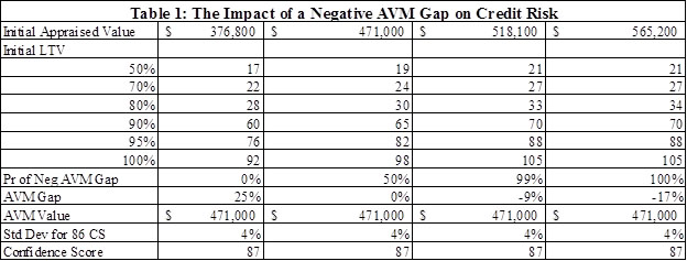
Now consider the first column in which the AVM exceeds the initial value of $376,800 by 25 percent. The probability of negative AVM gap in this case is virtually zero.  The credit risk on this loan is lower for each LTV relative to column two and the increase is 75 basis points for the two extreme LTVs in this case (92-17).

The more important results pertain to columns 3 and 4 in which the AVM gap is -9 and -17 percent of the initial appraised value. These translate into the probability of a negative AVM gap of 99 percent and 100 percent, respectively.  The CR spreads are predictably higher in column 3 than column 2, the base case. The differences range from 2 basis points for the 50 percent LTV to 7 basis points in the case of the 100 percent LTV. The final column shows virtually the same results as column 3, which is consistent with the fact that the probability of negative equity is virtually the same in both columns 3 and 4.

Is this a significant amount quantitatively? The present value of this difference is about 25 basis points. In dollar terms this amounts to about $1,230 in credit losses — .0025*.95* $518,100. This may seem modest but in comparison to the cost of an updated AVM, this is a substantial amount and likely to be money well spent by lenders to help insure against excessive initial appraisals on its residential loans.

Obviously, these results are based upon one specific property and set of loan assumptions. We also constructed the same example for an identical ARM with a 1 year rate adjustment period and the dollar amount of the losses due to a negative AVM gap were about 25 percent higher. More generally, the quantitative impact will vary with a number of traits in predictable ways. For example, loans with higher credit scores will lessen the impact of a negative AVM gap.

We also expect variations among markets in the quantitative impact of the probability of a negative AVM gap. One pattern that we also expect is that impact of the probability of negative equity to vary among markets. This example is based upon one property in Orange County, CA. Differences among markets are driven by local house price scenarios and other local market traits embedded in the CA Credit Risk Model. Though the quantitative effect varies among markets, the qualitative result is strongly robust. [2]

In sum, a loan with a higher initial value for a given loan amount may look to be less risky than a loan with a lower initial or appraised value for the same loan amount, but such a look may be deceiving if the initial value is inflated or upwardly biased. The CA Credit Risk model confirms and quantifies this important potential risk of mortgage lending.  Indeed, plans are underway to provide AVM clients with key summary results of the Credit Risk Model to help them use both the standard AVM results and the credit risk model results to prioritize property valuations most in need of additional scrutiny. This can be done by having the lender provide initial information of both the loan and the property. Alternatively, CA can provide the results for a stylized loan product for a particular LTV, credit score, and location.

Download a PDF file of this research paper here.