Modelling House Prices at the MSA Level Results and Implications for the Credit Risk Model

by Dr. James R. Follain and Dr. Michael Sklarz

Overview: The Importance and Challenges of Predicting Future House Prices

CA’s new Credit Risk Model (CRM) generates measures of the credit risk associated with residential mortgages. One summary measure is the Credit Risk Spread (CRS), which is the annualized value of the cost of borrower default. Like most models of mortgage credit risk, the CA CRM demonstrates that the CRS is driven by the initial loan to value ratio and the borrower’s credit score: higher initial LTVs and lower credit scores increase the CRS, all else equal. A key theme and a distinguishing feature of the CA CRM relative to most other models is the emphasis upon variations in the CRS among metropolitan housing markets. Markets in which the outlook for future house prices is strong have lower CR spreads relative to those with the future outlook of house prices is weak. A number of articles about the CA CRM are available on the CA web site.

The Credit Risk Model rests on two key assumptions. The first is that future house price movements will vary widely among local housing markets, which we define in the CRM as the metropolitan area. Absent such variation there is no motivation to measure variations in CR spreads. The second key assumption is that the processes underlying the predictions of future house price movements in the CRM are “reasonably” accurate. Again, if the model predictions of future house price movements prove to be quite poor, then the variation in the CR spreads will be driven by model error and not valid and measureable variations in the CR spreads among markets.

The first of these two assumptions is relatively easy to establish. For example, a recent article by Follain and Sklarz (2014) offers strong confirmation of the wide variations in house prices around the national average between 2005 and 2013. Of course, there is an abundance of other evidence to validate this assumption.

The second assumption is the more difficult one to establish. It is surely well-understood that predicting future house price movements is not an exact science. This is especially true about the ability of economists and others to predict extreme declines in house prices. Follain highlights this challenge and encourages economists to be more humble about our ability to predict extreme events. However, Follain and Giertz (2013), Miller and Sklarz (2013), Follain and Sklarz (2005) and others demonstrate that econometric models of house price movements at the local market level do tell us something of value and worthy of value in the measurement of local market credit risk.

The purpose of this article is to demonstrate some of the challenges in predicting house price movements at the local market level and some of the insights obtained from HP model predictions. This is done by examining one specific approach or model underlying the CA CR Model. The model is used to generate five year forecasts of house prices for a large number of MSAs. In addition, variations around the baseline forecasts (hp1) are used to generate six additional HP scenarios. One of these is the severe or stress scenario (hp7), which plays a critical role in the measurement of CR Spreads and the amount of capital that lenders need to hold for their investments in residential mortgages.

Description of the CA House Price Model and Key Assumptions Underlying the Model

The models consists of a single equation. The dependent variable is the natural log of the median sales price. The drivers of this measure of house prices include the lagged values of employment, household income, and the number of households, all of which are measured in natural logs. Two interest rate measures are also included: the level of the 10 year Treasury and the gap between the 10 year and 1 year Treasury rates. The final variable in the model is the index of US House Prices, as measured by FHFA’s repeat sales index. The estimated equation also includes MSA specific fixed effects, which capture the average gap between the level of prices in an MSA and the amount predicted by the economic variables in the model.

A key assumption in Model #1 is that the model is best estimated by pooling groups of MSAs. This is an intermediate approach between two extremes. One extreme would pool all MSAs and generate a common set of coefficient estimates for all MSAs. This runs the risk of imposing inappropriate coefficients for many or most MSAs. The other extreme is one in which the model is estimated separately for each of the 384 MSAs in the sample. This can result in less precise estimates due to relatively smaller sample size and omitting common ground among MSAs. Of course, choosing these groups is a judgment call. Our approach uses nine different groups of MSAs. Three are based upon employment growth between 1990 and 2010 and three are based upon the size of total employment in an MSA in 2000. The groups represent those above the 75th percentile, below the 25th percentile, and those between these two percentiles. Quarterly data from 1984 through to 2014:q2 and 384 MSAs are used for the estimation.

Coefficient Estimates

A key indicator of model performance is the sensibility of the estimates of the coefficients in the model. Variations among the coefficient estimates among the nine groups is expected and reflect traits of the groups not captured by the variables in the model. Table 1 contains key coefficient estimates.

Four lagged values are used for HH, HH Income, and Employment. The sums of the lagged values are presented in the table. HH Income and Employment consistently have positive coefficient estimates, as expected. The number of households, on the other hand, has both positive and negative estimates. The two interest rate variables also have both positive and negative coefficient estimates. With three exceptions, the coefficient estimates of the 10 year Treasury are positive and significant, though the magnitude varies substantially. The estimates for the difference in the T10 and T1 rates also vary widely. These results for the two interest rate variables are consistent with widely varying impacts of monetary policy on local housing markets. A consistently strong performer is the US House Price Index; indeed, all of the coefficient estimates for this variable are statistically significant. Lastly, note that the explanatory power of the equations is consistently high, i.e. R2 is .85 or higher for each group of MSAs.

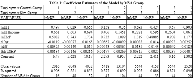
Overall, the coefficient estimates and the explanatory power of the model are judged to be reasonable or credible.

Examining Model Predictions for an In Sample Period

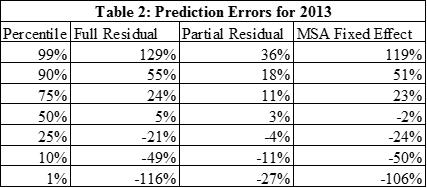
Other support for the predictions of the model can be obtained by examining its ability to predict future price changes. This is done by using the model estimates through 2011 to predict house price growth for 2012:q1 through 2014:q2. Table 2 contains a summary of key aspects of the average prediction errors for this period. The standard or full residual is computed as the difference between the actual value of lnMSP and the predicted value from the model (column 1). However, the estimation procedure allows this to be dissected into two parts. One is a more permanent MSA effect, which is estimated by the model and is constant over time for each MSA. The difference between the standard residual and the MSA fixed effect is labeled the partial residual and is designed to capture short term deviations of the model predictions that take account of this long term MSA fixed effect. The partial residual is in column 3 and the MSA fixed effect in column 4 of Table 2.

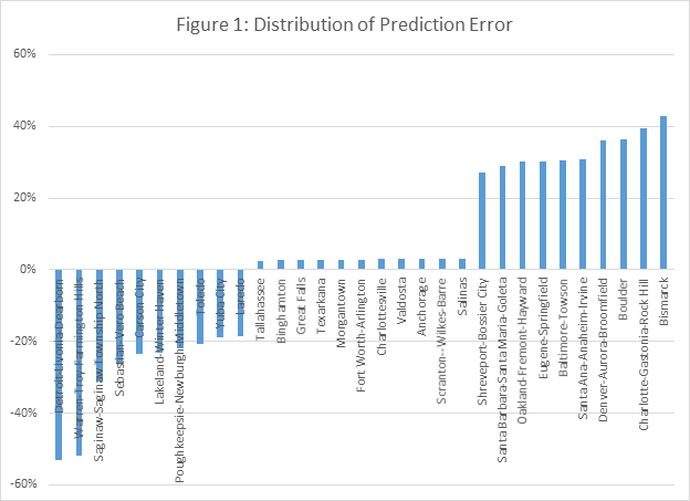
The median full residual prediction error is 5 percent and the variation around it is substantial. 50 percent of these prediction errors fall between +24 percent and -21 percent. The distribution of the partial residual error is more compact. The average is 3 percent and 50 percent of the MSAs are between 11 and -4 percent. This difference is driven by the wide variation of the MSA fixed effects. Figure 1 highlights the prediction errors for MSAs at the two extremes and in the middle.

FORECASTS

The ultimate purpose of the model is to generate future predictions of house price movements by MSA for a five year or 60 month period. Seven different scenarios are used by the CA Credit Risk Model. These include the baseline (hp1), a severe stress scenario (hp7), and five others distributed around the baseline. This section discusses the steps and assumptions used to generate these scenarios and insights they offer about which markets appear to be in store for substantial growth (Hot Markets) or decline (Cold Markets).

Step 1: Predict exogenous variables

The first step in the forecasting process is to generate predicted values for the exogenous variables in the model. A VAR (vector autogressive process) is used to generate predicted values for three of the exogenous variables: employment, households, and household income. This is a 3 equation model in which these variables serve as the dependent variables and the right hand side variables include 4 lags of each variable. A separate VAR model is estimated for each MSA individually. Our analysis of these predictions suggest they are quite reasonable. The average cumulative predicted growth rates in these variables are 7 percent for employment, 5 percent for total households, and 13 percent for median household income.

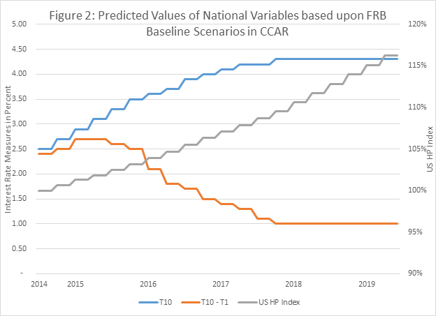
The three national variables – the 10 year Treasury, the gap between the 10 year treasury and the 1 year treasury, and the US HP index – are based upon recent national scenarios provided by the Federal Reserve Board for use in its evaluation of large banks in its CCAR Program. The baseline line scenarios are quarterly and extend to the end of 2017. We extend these further to 2019:Q2 by using the 2017:Q4 values for the additional six quarter. The scenarios do not include a one year treasury but do include a 30 day Treasury. The 1 year treasury is defined for the forecast period to be the 30 day Treasury plus 10 basis points. The FRB scenarios also include a projection of the national house price index. Plots of the values utilized in the forecasts are contained in Figure 2.

The 10 year Treasury is projected to grow from 2.5 to 4.3 percent. The gap between the 10 and 1 year treasury narrows to 1 percent. The US House Price index grows rather steadily by 15 percent. This includes 4 percent per year in 2018 and 2019.

Specific Forecasts

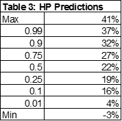
Table 3 offers a summary of the cumulative predicted house price changes from 2014:q3 through 2019:q2 for the baseline scenario. The median cumulative price change is 22 percent, which is about 4.5 percent per year. The most optimistic predictions call for 6 percent or more per year. About 10 percent of the MSAs fall into this category. At the other end of the spectrum, 10 percent of the MSAs are projected to grow at 3 percent or less per year. 50 percent of the MSAs are predicted to grow between 19 and 27 percent during the five year forecast period.

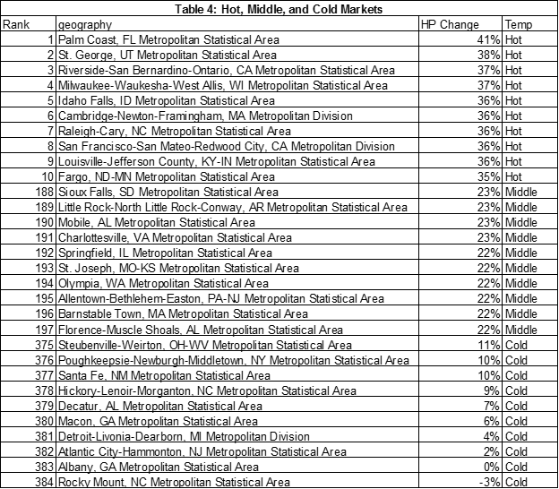
More insight about the distribution of these predictions is obtained by focusing on the specific MSAs with the largest predicted changes (Hot markets), those with the smallest (Cold markets), and those in the middle. Table 4 presents the predictions for the 10 hottest, 10 coldest, and 10 around the middle. Each group contains MSAs from different parts of the county.

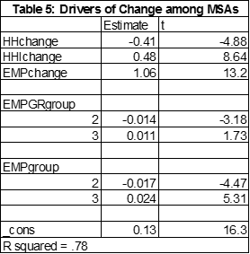
Additional insights about the distribution of these predicted changes can be obtained by a simple regression that explains the cumulative growth rate at the MSA level during the forecast period as a function of the cumulative growth in the three main drivers – employment, household income, and the number of households. The regression results are in Table 5.

Employment is the most important driver among this group of variables. The change in median household income also has a positive and statistically significant impact. The number of households actually reduces the change in house prices, all else equal. Predicted price growth is largest for the largest group of MSAs and smallest for the middle group of MSAs in terms of employment size. Predicted price change is largest for the fastest growing group of MSAs.

Generating other Scenarios

Another critical part of the house price predictions for the Credit Risk Model entails the generation of six other scenarios around the filtered baseline prediction. One of these is the severe or stress scenario (hp7), which is used to define the amount of capital required by a lender to protect against an extreme decline in house prices. For example, the Fed’s prediction of this “severely adverse scenario” calls for a monthly decline of 25 percent reduction in national house prices from the end of 2014 to 2016:q1. We offer a definition of the stress scenario that varies modestly among markets and is a constant rate of decline per month. For those outlier MSAs with the predicted baseline price changes 5 percent or less, the monthly stress scenario is a .2/60, which generates a cumulative percentage decline of about 18 percent. For those MSAs with predicted baseline changes of 30 percent or more, hp7 calls for a monthly decline of .30/60, which generates a cumulative decline of about 26 percent. For all other MSAs, the stress scenario calls for a monthly decline of .25/60, which generates a stress scenario of about 22 percent.

The other five scenarios are designed to surround the filtered baseline and incorporate the important point that mortgage credit risk is driven not just by baseline and stress scenarios but also by modest variations around the baseline. This follows from the widely accepted factoid that an increase in house prices has little or no effect on default but a decrease of the same amount would. The other five scenarios are designed to capture the impact of this asymmetry.

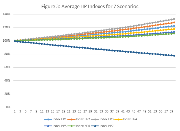
A monthly prediction error is assumed to be .0066, which is consistent with a quarterly model error of about 2 percent per quarter. This is consistent with the prediction tests above using the partial residual error. The monthly equivalent of this error is 0.006667 per month (.02/3). Two scenarios – hp2 and hp3 – are set at .1 and .2 of the error above the filtered baseline. Two scenarios are set at .1 and .2 of the errors below the filtered baseline – hp4 and hp5. The final one is another negative one and is set at .25 of one error below the filtered baseline. The house price indexes based upon these seven scenarios are in Figure 3. The monthly changes in these indexes are fed into the Credit Risk Model and used to calculate the credit risk in these MSAs.

Summary and Conclusions

This report has laid out the processes used to generate future house price projections to be used by CA’s Credit Risk Model. It is based upon a single equation model in which house prices at the MSA level are driven by a set of local market conditions and a set of national indicators. The model is used to produce 5 year forecasts of future house price movements for seven scenarios; one is the baseline, one is the stress scenario and the other five span the baseline scenario. We judge the results to be credible. It seeks to highlight the many assumptions and challenges in generating future house price projections. The results demonstrate two high level points. First, predicting future movements in house prices, especially extreme increases and decreases, is very challenging. As Follain (2013) argues, economists need to be especially humble about our ability to predict the future, especially extreme events. But, secondly and on the other hand, models based upon sound economic theory and historical data can tell us something about the future. Among these is the strong expectation that future house price patterns have historically been driven by local market conditions and can vary widely. As such, we feel comfortable in rejecting the proposition that future house price movements will be highly similar among markets. This is where the Credit Risk Model can be of help to lenders and investors in residential mortgages because it incorporates plausible estimates of future house price movements into the calculation of credit risk spreads.

Improving the process to estimate future house prices is an ongoing process. Among the most important areas to consider is the residual from the first stage regression, which has a major impact on future house price movements. While the basic theory and core results confirm its role, the magnitude of the size of the residual among markets is shown to be substantial. Options to better measure it and reduce the extreme values is a priority we will be considering. Another possibility is to consider additional variables like residential rent and alternative groupings of MSAs.

Download a PDF file of this research paper here.