by Dr. Michael Sklarz and Dr. Norman Miller | October 16, 2017
Download a PDF file of this research paper here.
Introduction
As of the fall of 2017, the media and many housing analysts seem to have the view described below:
“Every city I visit around the world, I hear the same story: Housing is unaffordable. Millennials, even those with good jobs, are struggling to get into the housing market, and they are not the only ones.”
– Richard Barkham, Global Chief Economist for CBRE.[1]
Perhaps we need a new definition of housing affordability or perhaps we need to ask Dr. Barkham to visit a few more modestly sized cities, although he does conclude there is no housing bubble looming. Still others have been singing the same song for decades, that we are in a housing crisis based on concerns over middle and lower income households not being able to afford rent or to purchase a home. The view that we are continually in a housing crisis is a result of a successful economy and American wealth creation that has pushed up prices for most owner-occupied-households, while simultaneously blocking smaller and more affordable housing supply choices via grass roots political opposition. While the concerns over housing affordability date back for hundreds of years, here are just a few discussions dating back three and a half decades.
In January of 1982, Ira Lowry in a Rand note for HUD, stated that “Recent public discussion of the ‘rental housing crisis’ reflects two widespread beliefs: (a) that rental housing is in short supply, and (b) that rents have consequently risen faster than renter’ incomes. These perceptions underlie recommendations for measures to increase the supply of rental dwellings by subsidizing new construction and restricting conversions to non-rental uses; measures to restrain rent increases; and measures to subsidize the operation of rental properties for low-income tenants. Analysis of recent price changes …yields strong evidence that market conditions have been badly misinterpreted.” [2]
In the year 2000, the Harvard Business Review, published “No Place Like Home: America’s Housing Crisis and Its Impact on Business” [3] Gary Emmons stated “In many parts of the country, housing costs and shortages have begun to show signs of adversely affecting corporations, workers, and local economies. Affordable housing — such as Boston’s Orchard Gardens, — is increasingly scarce. How serious is the problem?…It’s a tale of two Americas, the best of times and worst of times, if you’re a consumer in the current U.S. housing market. On the plus side, thanks to the 1990s’ economic boom, some two-thirds of Americans, more than ever before, currently own their homes. At the same time, housing of all kinds — for buyers and renters — has become more expensive precisely because of the country’s prosperity.”
More recently, in 2016, Glen Kelman, CEO of Redfin in a report for CNBC, stated: “Want to help the middle class? More houses, please” …“The U.S. is building new homes at about half the historical rate, and it’s causing our cities to become unaffordable.”[4]
The reality is that as long as our housing market does well for those that are currently owners, it will challenge some to enter the market, and as long as supply barriers remain high in some markets, rents and prices will often exceed inflation rates. Yet, for most of the US market, the reality is that housing remains affordable. Here we propose a new measure of housing affordability that considers various price tiers as well as property taxes, which vary greatly by market.
Traditional indices of home affordability, like the well know ones published by the National Association of REALTORs® (NAR), use median household income and median prices as the primary criteria for affordability. This median-median approach ignores the lower than average loan to value ratios observed on the most expensive homes, biasing any median index in a negative direction.[5] Such a median-median approach, also ignores the distribution of home prices observed. Here we explore the distributions of home prices by slicing the home prices into deciles, where each decile contains 10% of the homes sorted by selling prices each year for each CBSA. Next, we examine the proportion of median incomes required to support mortgage payments, not just for the median home, but for other lower distributions. This perspective is more in line with what could be called an “entry level housing affordability index” and that is often the concern, when stories of housing being unaffordable abound.
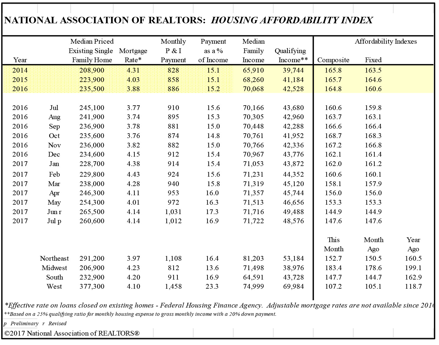
In markets like California, or Hawaii with severe supply constraints, we often hear that we are in a “housing crisis” and not producing enough of the smaller and more affordable housing units. This remains a valid concern. But, for the nation as a whole there is no housing affordability issue. The overall U.S. Housing Affordability Index in the latest reporting months is 147.6, which means that the average for all CBSAs of median income required to buy a median priced home in the US is just under 70%.[6] This suggests that, on average, housing is affordable. When we define entry level housing as something under the median price for a given market, we find even less of a problem in most markets. Even some expensive markets are still affordable, if households can lower their aspirations to these lower priced tiers.
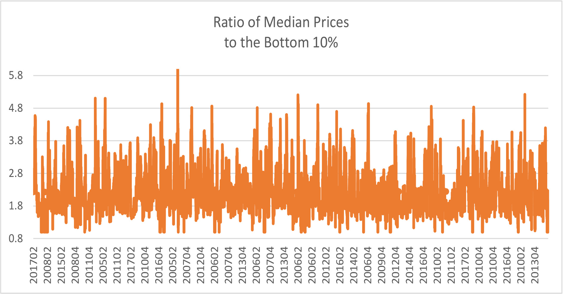
We will show required income ratios for a number of sample markets, but another part of the story is that price to income ratios are higher than ever and that the lowest priced owner tiers have done worse than upper tier housing segments. It is also true that many lower tiered owners lost homes due to high LTVs during the housing crisis. Yet, since 2007 the ratio of median prices to the bottom 10% decile has been rather steady at 2.2.
Below we start with a sample of home sold prices shown in deciles. We follow this with some affordability calculations.
Home Prices Segmented by Deciles
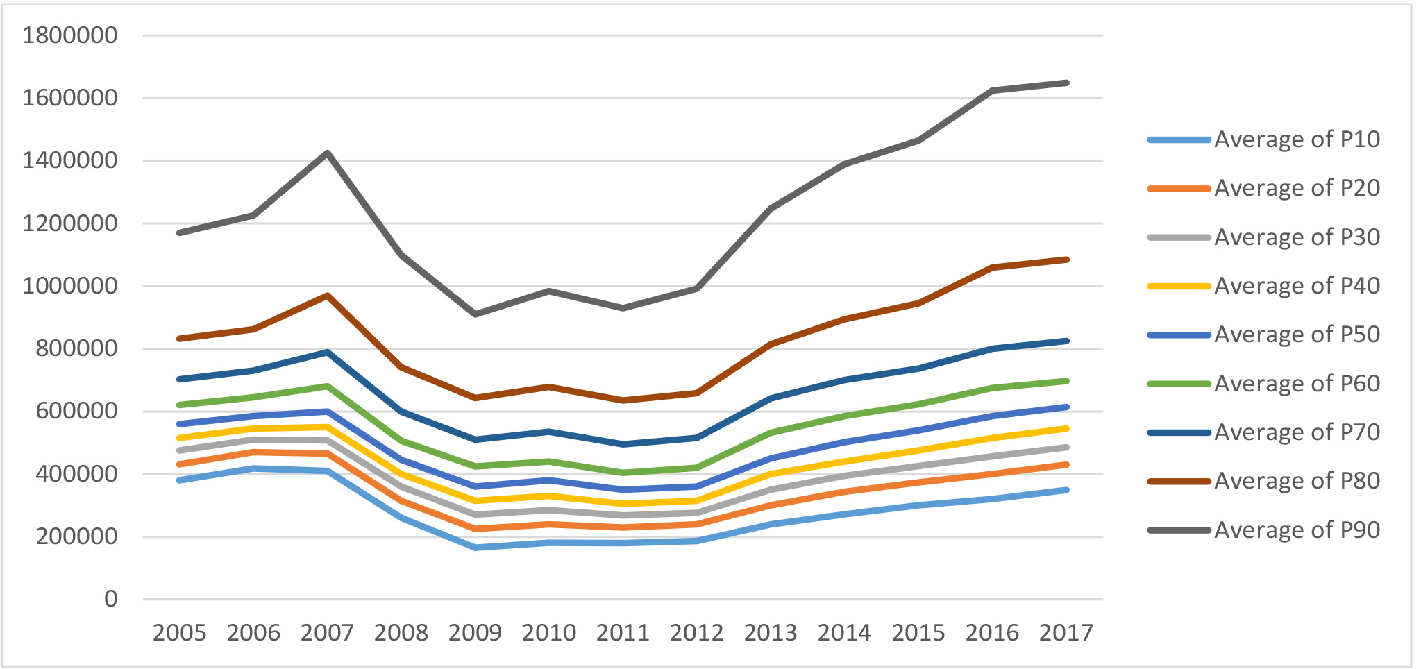
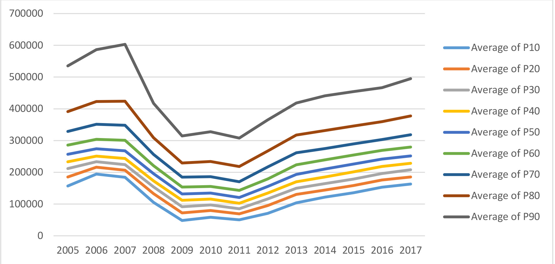
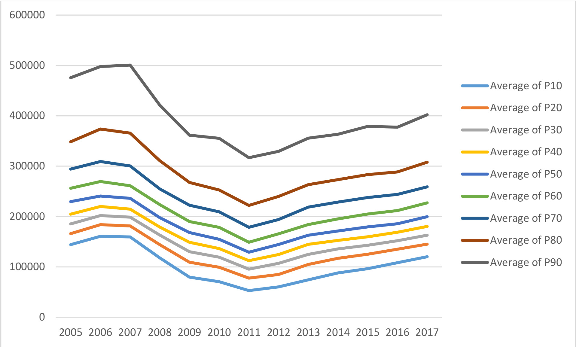
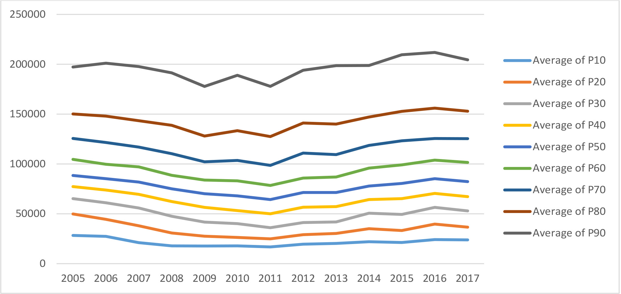
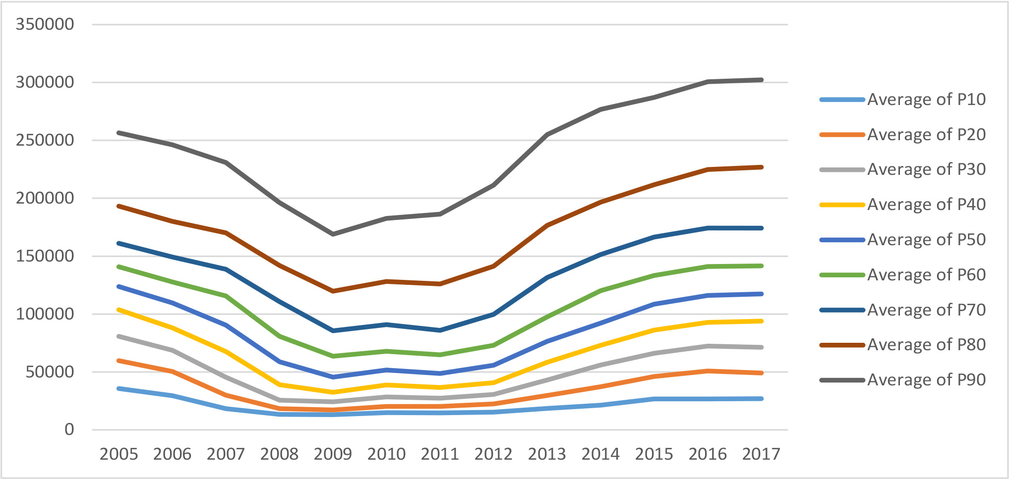
We start with some of the highest priced markets like San Francisco and Los Angeles, shown in Exhibits 1 and 2. For both of these markets we notice that the spread for the higher priced markets has increased since 2010. This will drive up median prices yet few households can afford such upper tiered homes without substantial equity. Note also that Los Angeles was more affected by the housing crash of 2008 than San Francisco.
Exhibit 1: San Francisco Metro
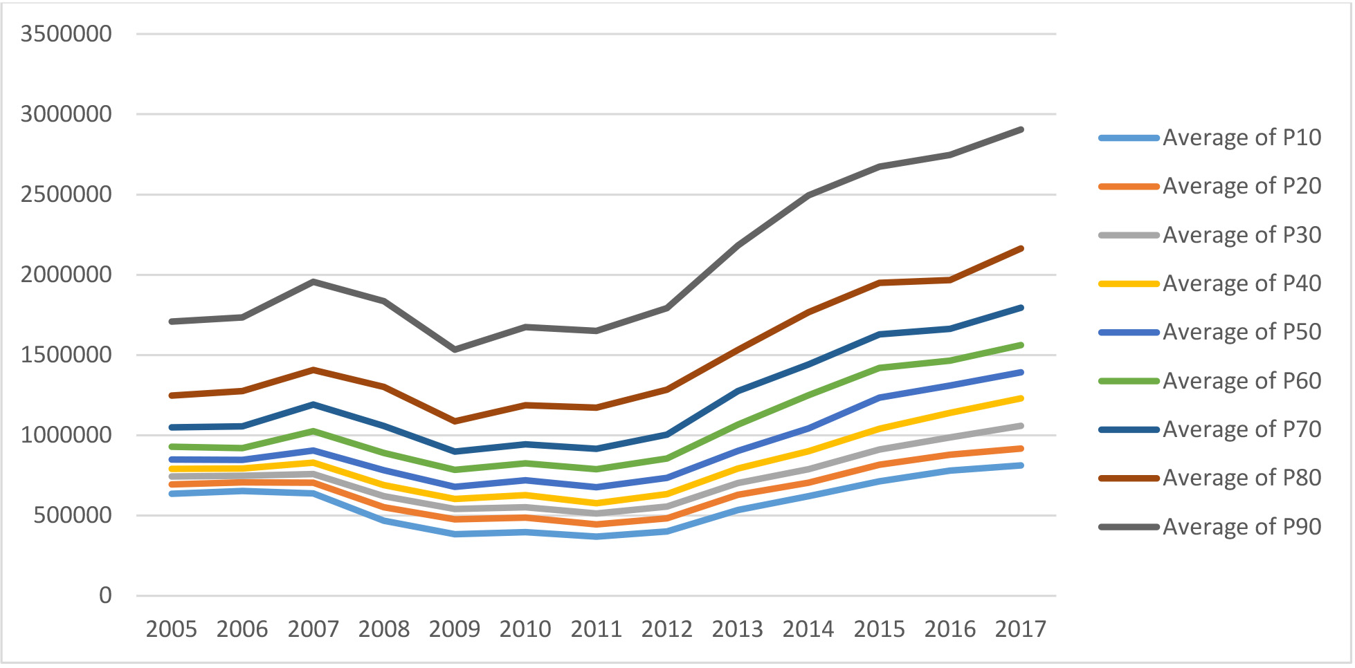
Exhibit 2: Los Angeles Metro
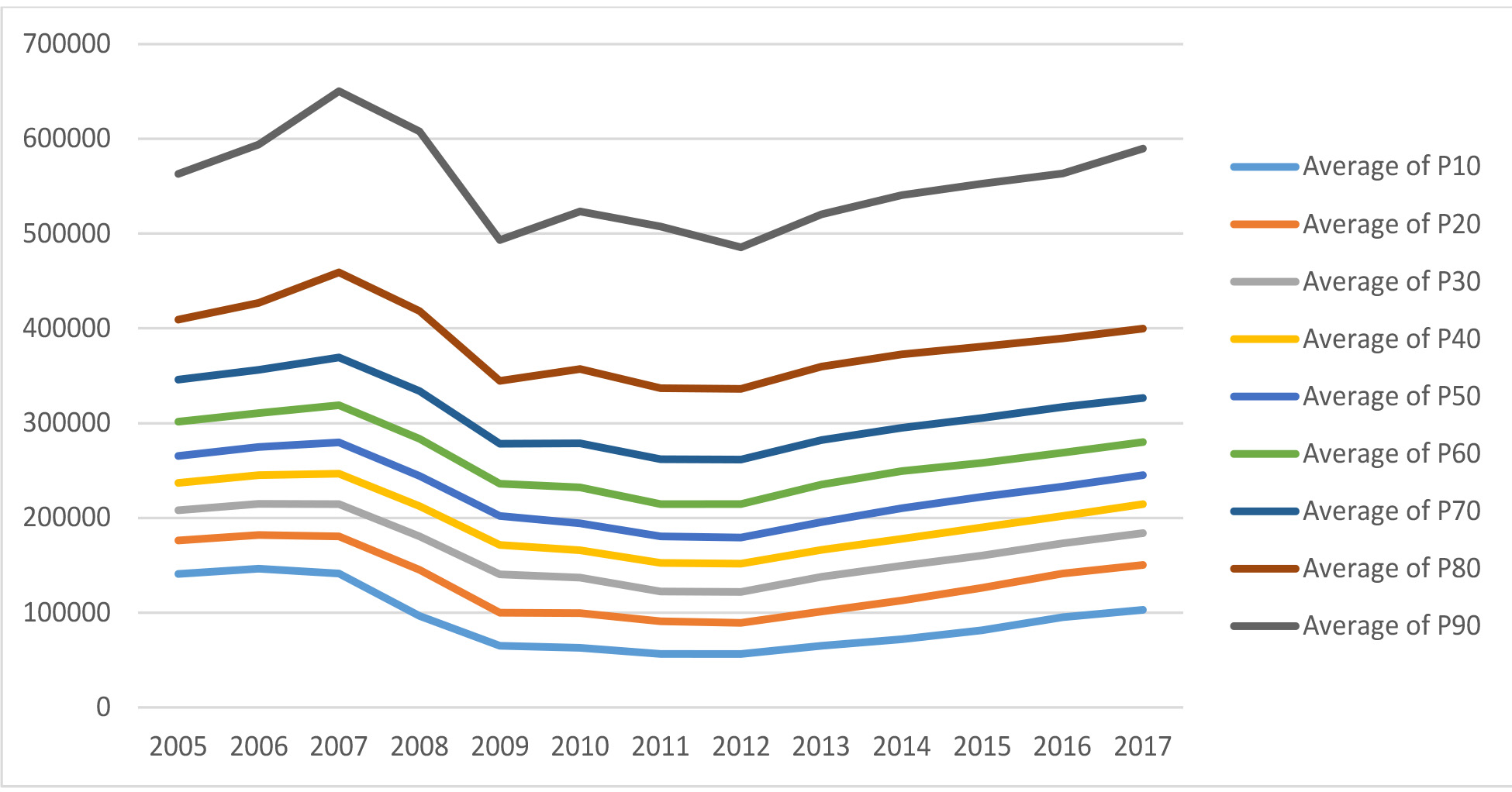
Despite substantially lower prices in Chicago (Exhibit 3) compared to San Francisco, we note again the large spread of highest price tier compared with the others, below.
Exhibit 3: Chicago Metro
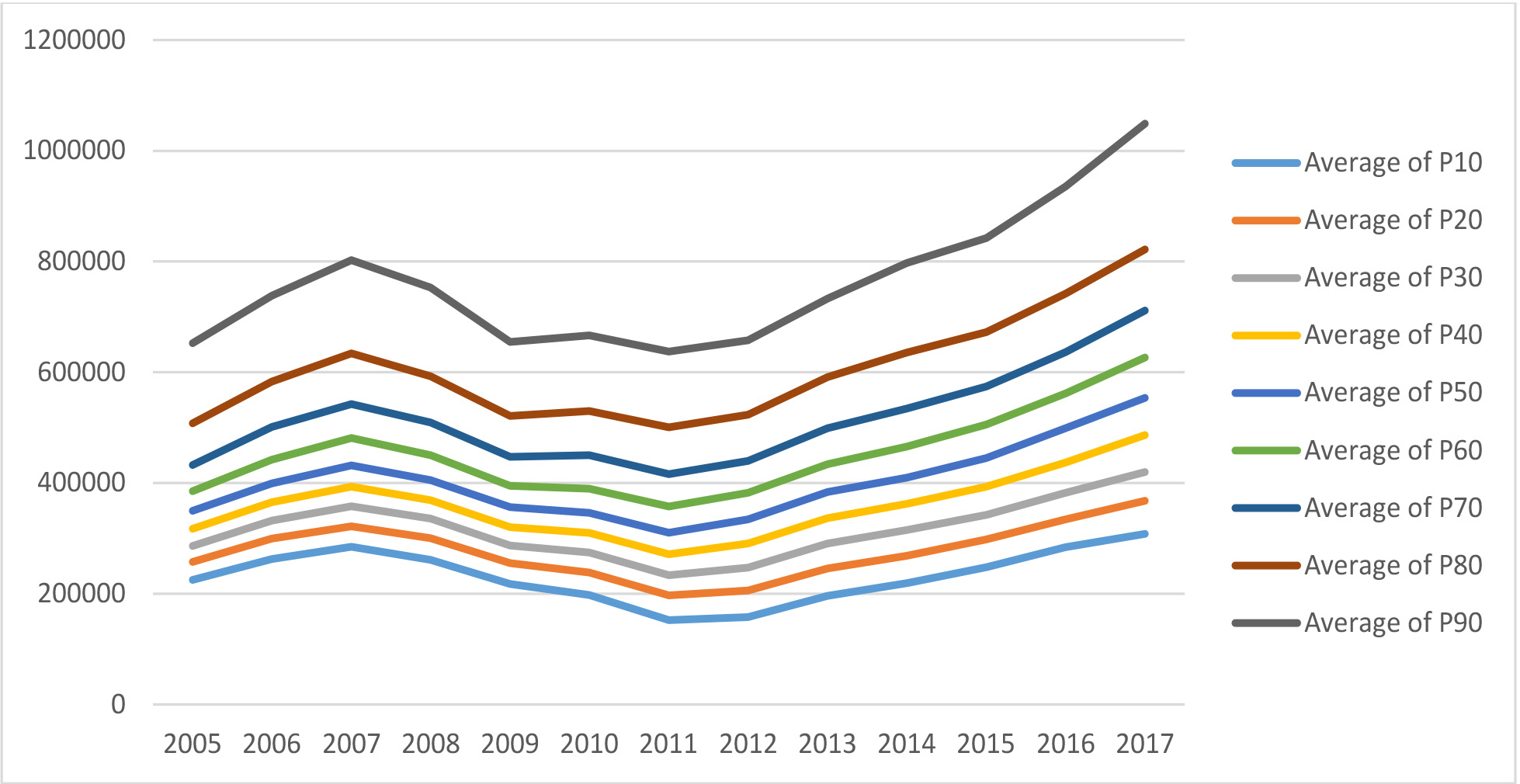
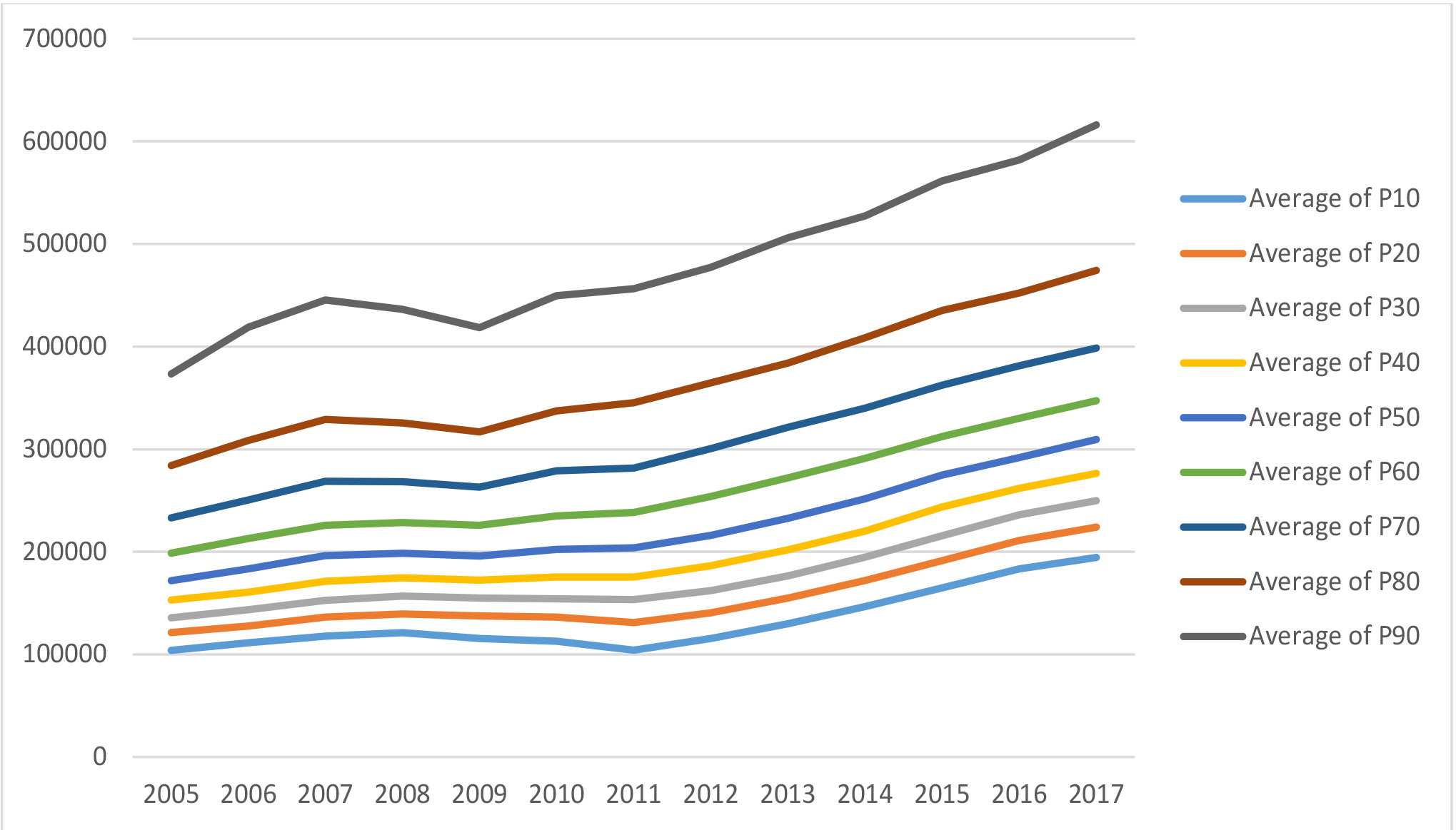
Next, we show Seattle (Exhibit 4), a market that started in 2005 with slightly higher median prices as metro Chicago, but has risen much faster and much higher. Note that all priced tiers have done well but the upper priced tiers have moved up relatively more than the average.
Exhibit 4: Seattle Metro
Phoenix (Exhibit 5) was a market severely affected by easy credit and high LTVs in the early to mid-2000s period and we see that all price segments were severely impacted by the downturn. The upper priced markets moved down faster and up faster than the lower segments with most segments moving in parallel.
Exhibit 5: Phoenix Metro
Also in Arizona, we examine Tucson below (Exhibit 6). Tuscon has yet to recover from the price declines of 2007 through 2011. The relative decline was similar to Phoenix but took longer to play out.
Exhibit 6: Tucson Metro
One market that never dipped, even during the national housing crisis was San Antonio. TX, (Exhibit 7). Prices were and remain affordable. Austin, TX, shown below (Exhibit 8) a more expensive market which also fared well with slight dip and pause.
Exhibit 7: San Antonio Metro
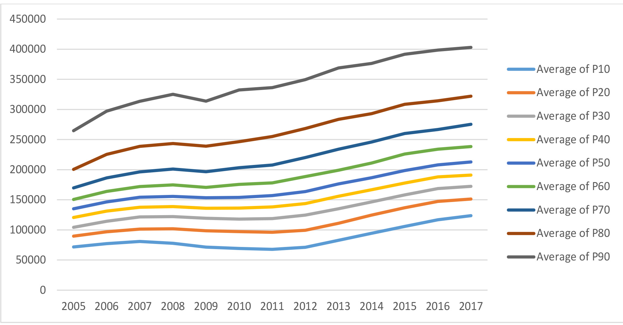
Exhibit 8: Austin Metro
Last, we illustrate some Midwest markets with less vigorous economies like Youngstown, Ohio, (Exhibit 9). Here we see low prices, highly affordable, and with historically modest appreciation. In real terms, adjusted for inflation, Youngstown prices have actually declined since 2005.
Exhibit 9: Youngstown Metro
Detroit (Exhibit 10) is an interesting market that was severely affected by the housing crisis and the lower price tiers almost collapsed upon one another. Yet, this market has rebounded significantly and remains very affordable.
Exhibit 10: Detroit Metro
Comparing the slope of the price tiers
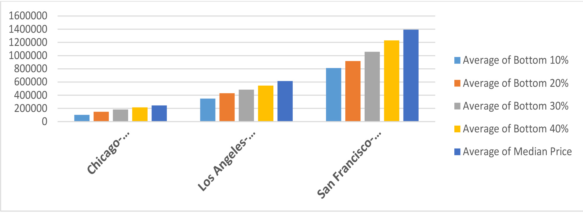
Below in Exhibit 11 we compare the ratio of home prices by tier for three housing markets and here we see increasing slopes of median to lower prices from fairly flat Chicago to San Francisco. These results seem correlated with land values, economic vitality and great global locations that attract buyers from all over the world, but more research is required to fully explain the patterns.
Exhibit 11: Slope of Price Tiers for Three Sample Metros
While it looks as if many markets have witnessed higher priced markets doing better than lower priced ones, for the nation, as a whole, median prices have not risen more than seen in the lowest price tiers. Below, in Exhibit 12, we show the ratio of these median prices to the lowest priced tiers.
Exhibit 12: Ratio of Median Prices to Bottom 10% From 2007 through Mid-2017 Nationwide
Affordability Calculations Based on Median and Lower Priced Tiers
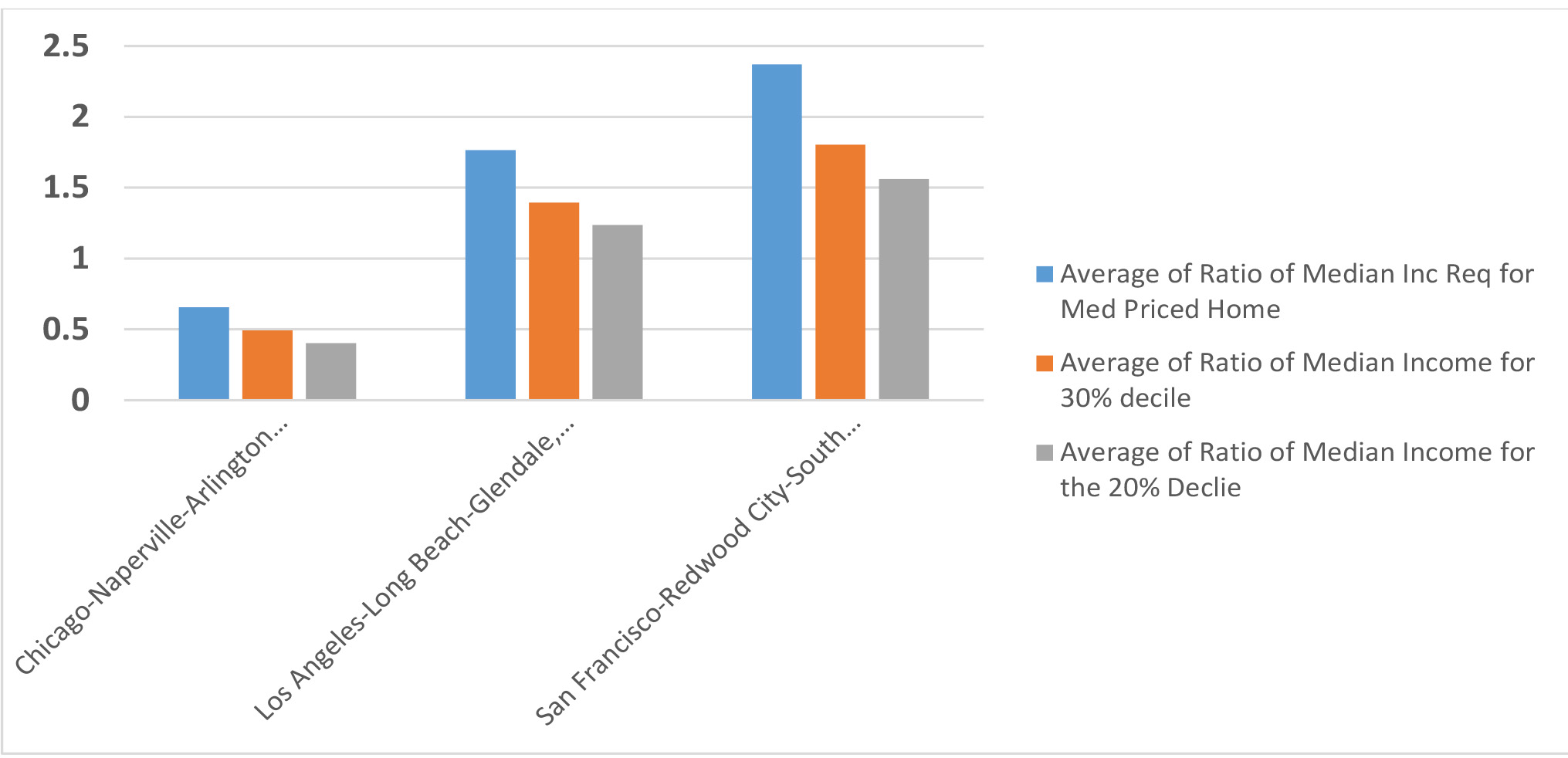
Instead of a traditional median household income relative to a median home price approach for affordability ratios, here, in Exhibit 13, we see how much of the median income is required to buy 1) the median priced home, 2) the bottom 30% and 3) the bottom 20%. The story here is that many markets contain quite affordable housing, even the Chicago metro, a large city, but one that has allowed increased densities over time.[7] When using the NAR’s criteria of a maximum of 25% of income for mortgage payments, we see that Los Angeles’ entry level housing based on the 20% bottom decile requires 120% of median income and if we used 30% of income instead of 25% for the maximum allocation of income to mortgage payments, the ratio would be 100%.
We are suggesting that affordability could be redefined to reflect more entry level housing based on a 20% or 30% decile home price tier. On this basis, it is possible for most households to buy into most US housing markets, albeit not a coastal supply-constrained high-end product market.
Exhibit 13: Ratio of Median Income Required to Buy Median Priced Homes, 30% Price tier homes and 20% Price tier homes
One counter argument to the fact that affordably priced housing tiers do exist in many markets, even where the top 10% of the market is quite unattainable, is that these affordable markets are not within good school districts. That would instead divert these households to rent in better school districts should no housing be affordable there. School districts and their impact on housing prices will be explored more in another white paper. Yet, in large metropolitan areas some lower priced housing may be attainable with acceptable school districts allowing an entry level affordability ratio to be pragmatic.
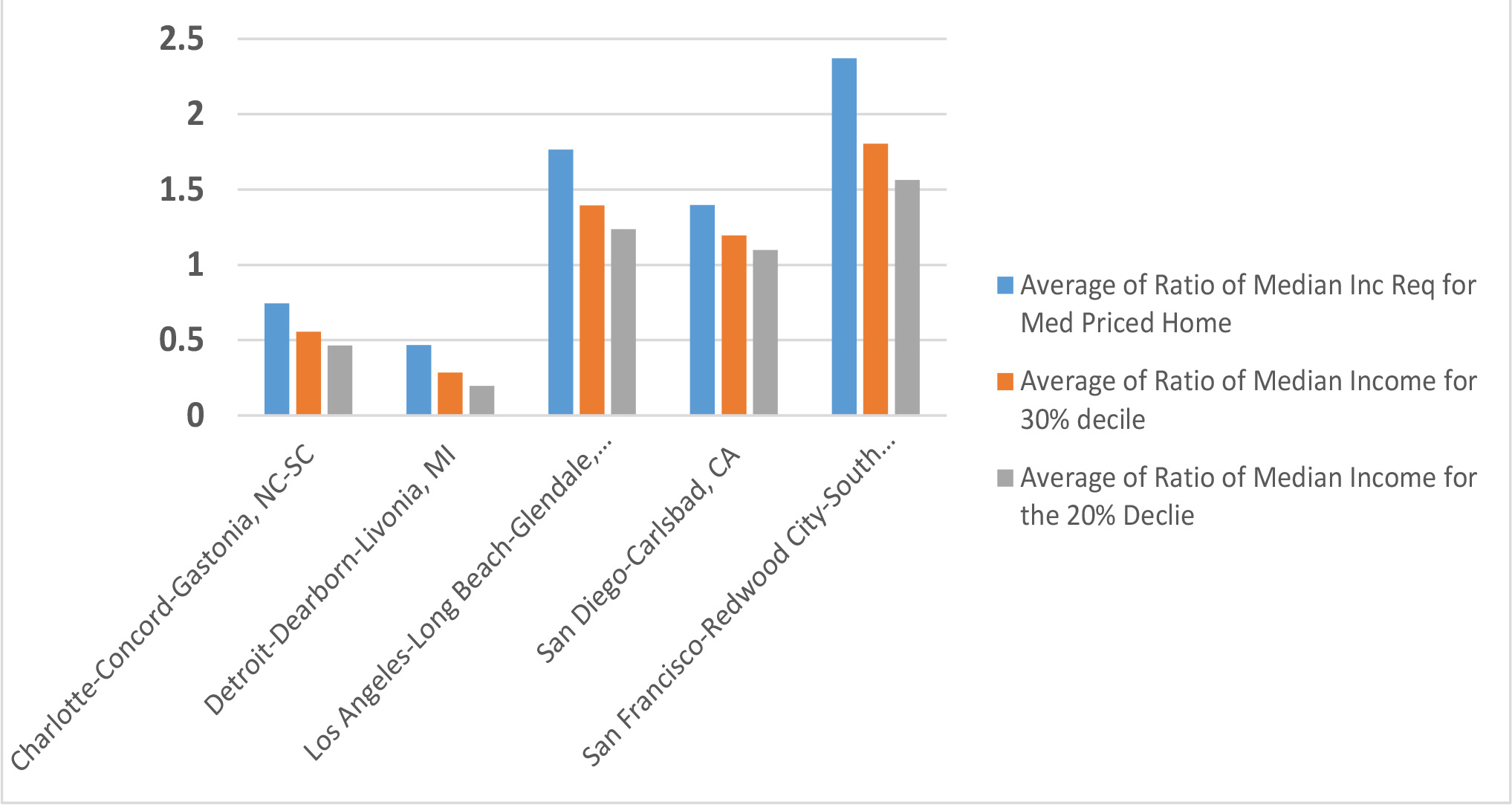
Below, in Exhibit 14, we retain San Francisco as a reference point but add the high-priced markets of Los Angeles and San Diego along with the lower priced markets of Detroit and Charlotte metros and repeat the same exercise of answering how much of the median income is required to buy the median priced housing, the 30% tier and 20% tier. Here we observe San Diego as almost being affordable at the 20% price tier level and highly affordable markets in the lower priced tiers.
Exhibit 14: Ratio of Median Income Required to Buy Median Priced Homes, 30% Price tier homes and 20% Price tier homes With Some Lower Priced Markets
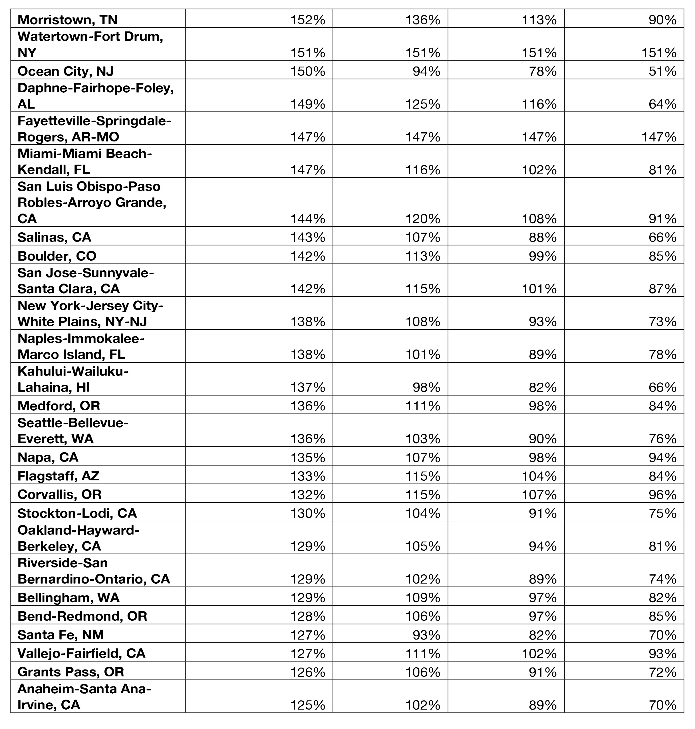
In the next set of Tables, we repeat the affordable calculations for 1) the median home price, 2) the 30% priced tier, 3) the 20% price tier and last, 4) the bottom 10% price tier. The top least affordable and most affordable CBSAs, out of some 380 markets, are ranked in the nest two tables.
In the least affordable markets we often observe supply constraints with high land values and sometimes high development fees, but there are exceptions, where incomes are simply very low.
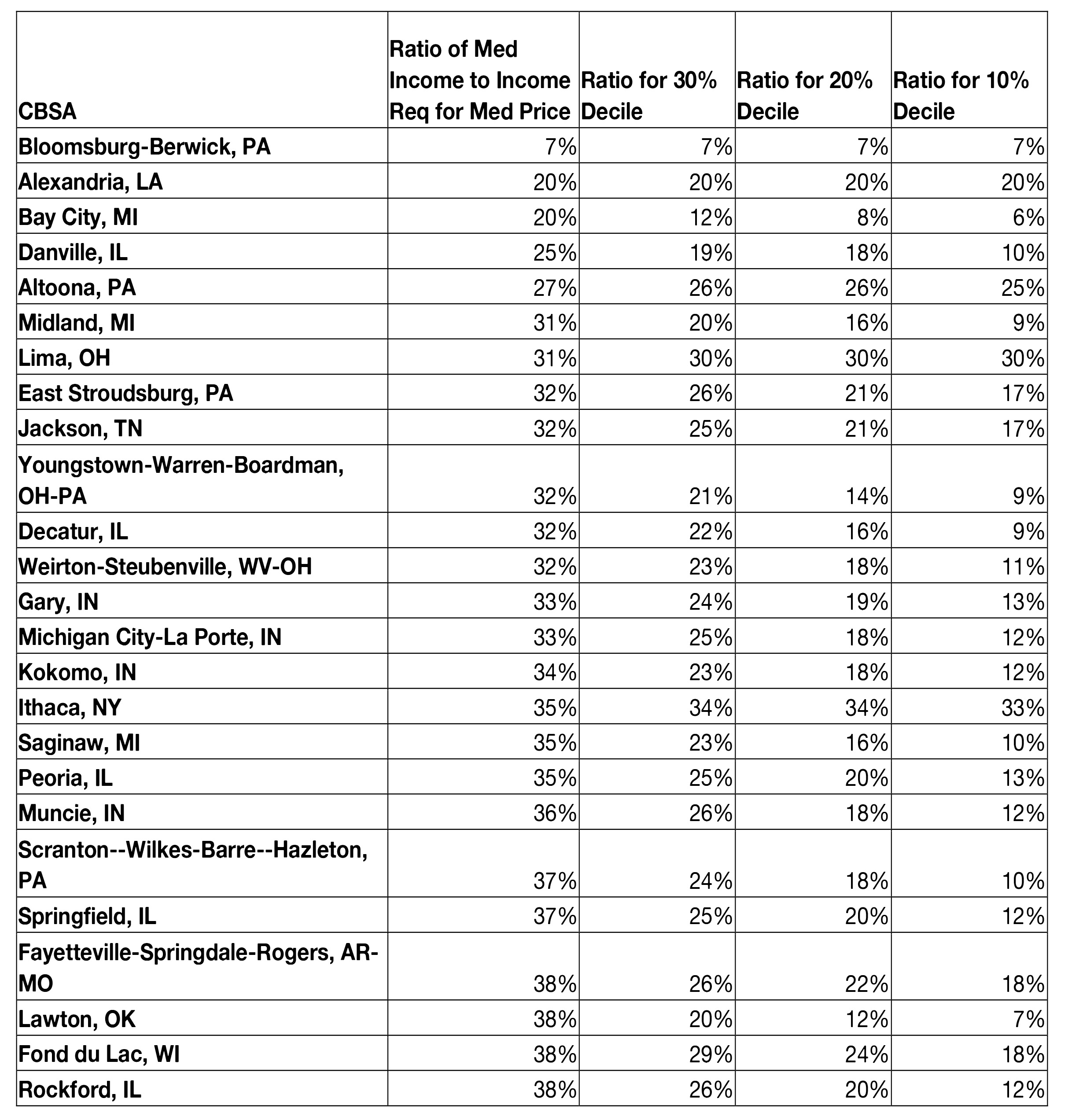
In the most affordable markets, we see that generally prices are low and it takes very little of the average household income to pay for housing. These markets are also relatively older, sometimes plagued with sluggish economies that have resulted in little population and employment growth.
If we utilized the lower decile price tiers the result is that some markets now deemed unaffordable with median income, like Miami, FL are affordable. This holds true for markets like Seattle, Ocean City, NJ, and Sante Fe, NM as well.
Table 1: Least Affordable Housing Markets Based on Simple Ratio of Required Percentage of Median Income to Median Price or Decile Shown
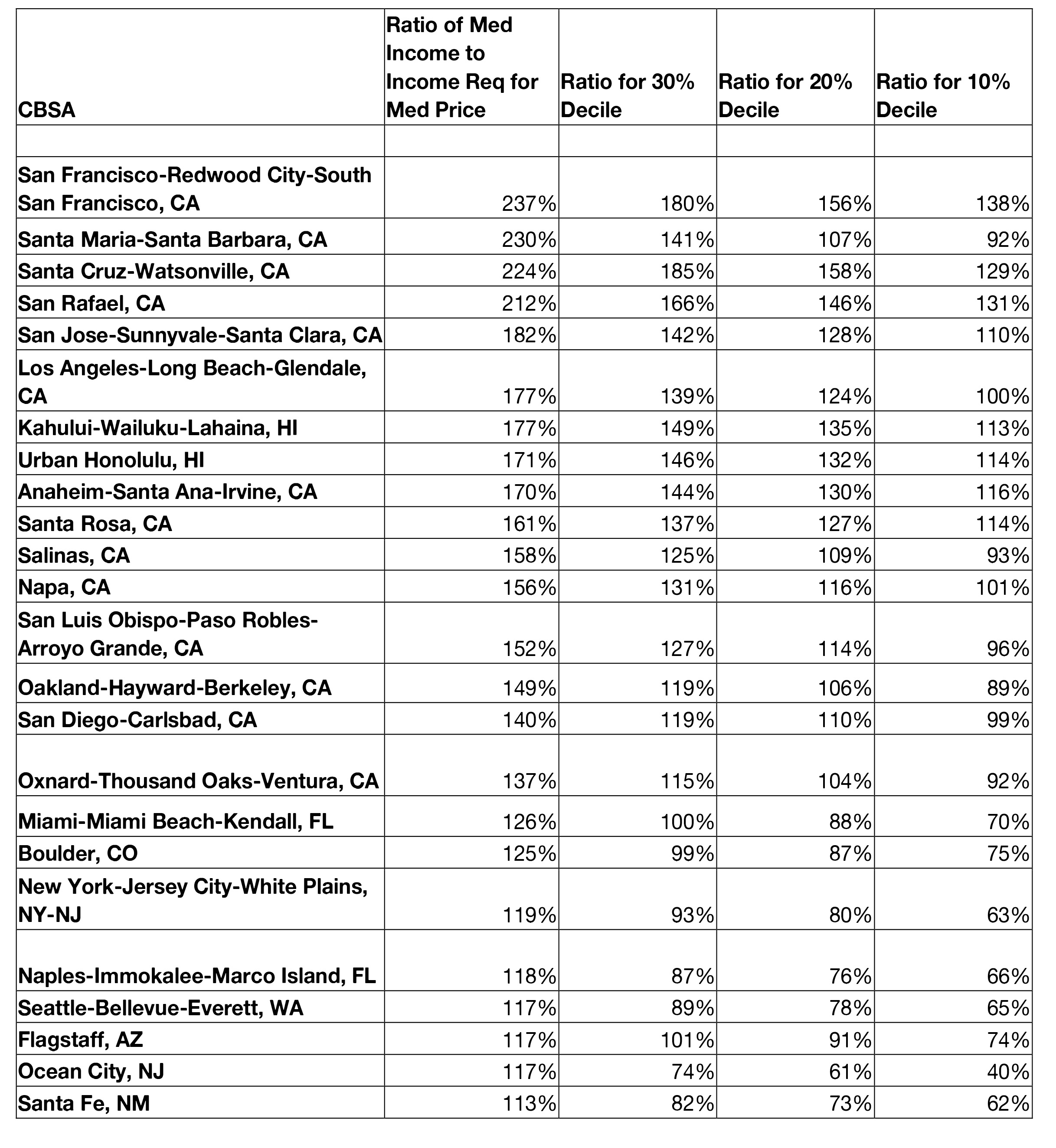
Table 2: Most Affordable Housing Markets Based on Simple Ratio of Required Percentage of Median Income to Median Price or Decile Shown
Affordability Results Based on only Mortgage Payments, Prices and Incomes
Most US housing markets are affordable, as of fall-2017, based on current mortgage rates, home prices and median household incomes. Coastal markets have tended to be less affordable for decades, and this is unlikely to change given the political resistance to any sort of increase in the density of proposed development, which is essential to lower housing costs. Expensive land can still co-exist in a market with more affordable housing and we see this played out in cities like Chicago, where relatively high densities are permitted in the central city.
We propose a new entry level housing affordability index based on no more than the 30% level of prices in any given metro. Some of those markets that are not affordable using median prices and median income may be attainable if we redefine affordability based on entry level housing at the 30%, 20% or even 10% price tier level, although some households will defer ownership rather than accept poor school districts or other negative externalities. Here we have examined affordability from the point of view of pricing by price tier, and based on income and mortgage payments. Next, we will incorporate the impact of property taxes and how effective property tax rates affects affordability.
Incorporating Effective Property Tax Rates
Effective property tax rates are defined as the actual property tax paid divided by the property value. We have used the Collateral Analytics AVM (Automated Valuation Model) to estimate property value and then calculated this ratio for all CBSAs. The average for the entire US is 1.068%. This suggests that a home worth $100,000 will pay on average $1,068 per year in property taxes. A home worth a million will pay $10,680 per year. The importance of property taxes as a source of local revenue varies by market and state. Some states rely more on sales taxes, others on income taxes and some on property taxes. For example, Hawaii relies less on property taxes and has the lowest average property tax rate as a percentage of value. New Jersey is on the other extreme with very high property tax rates. In further research, we will examine if some states have so significantly affected affordability that they actually depress property values. For now, we will simply incorporate the effective property tax rates into our affordability calculations. In Table 3 below, we show the average property tax rates as per the assessors, by state.
Table 3: State Rankings of Effective Property Taxes: Source: John S Kiernan, Wallet Hub, March 1 2017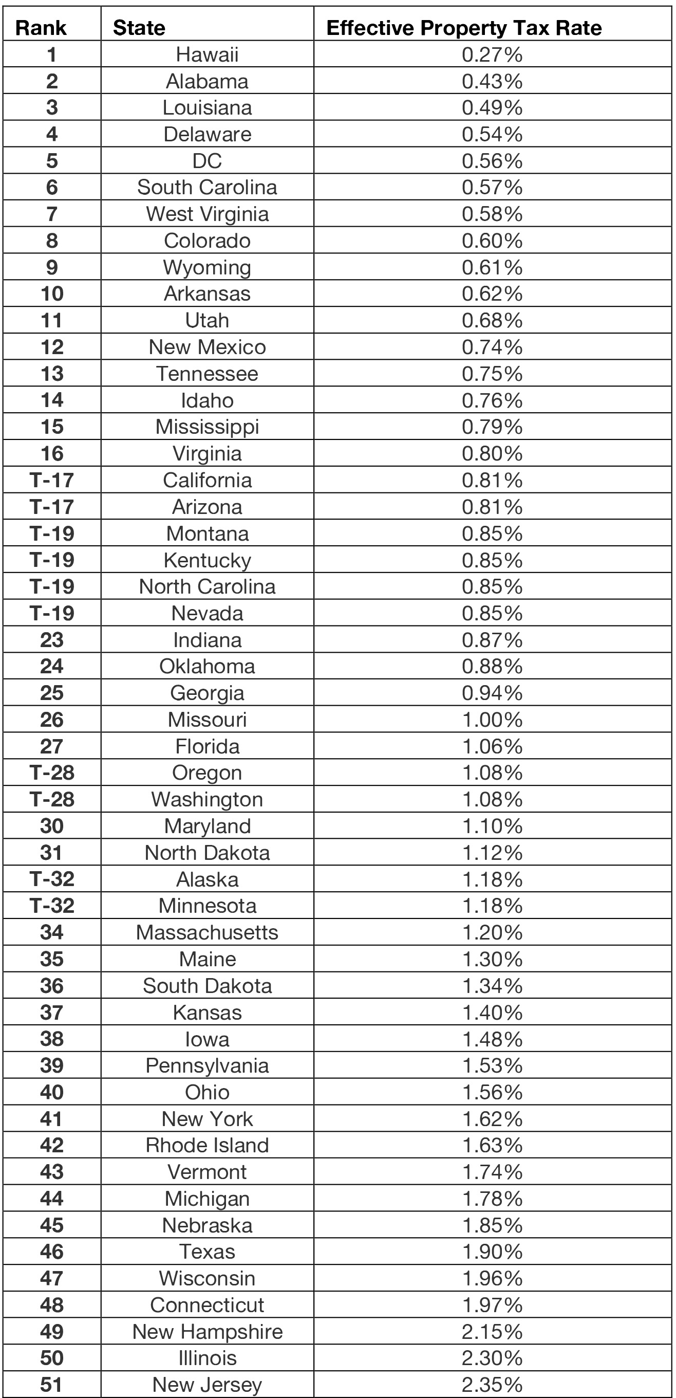
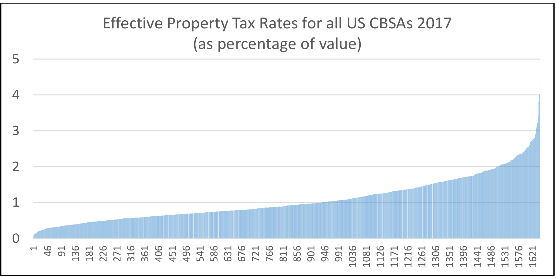
When analyzed at the CBSA level the variation of property tax rates as a percentage of value is even greater, as one would expect. In Exhibit 15 below, we show the variation of effective property tax rates for all the US CBSAs. Again, the average is 1.07% but the variation is quite large. At the low end are markets like Crossville, TN at .08% and Mount Sterling, KY at .11% where perhaps the updating of values might lag and the property tax rates are low. At the high end are markets like Great Bend, KS, at 4.48% and Altoona, PA at 9.03%. Altoona, PA has been deleted from the Exhibit below as a possible outlier.
Exhibit 15: Effective Property Taxes for US Cities
For every CBSA the average effective property tax rates are incorporated into affordability by adding the percentage of value required each year in property tax payments. This percentage is added to the annualized mortgage payment percentage and both are considered in the calculation of required income. Here 28% of median household income is used for a housing available funding of these two expenses. Last, we take the percentage of median income times 28% that is required for a 30% housing price tier home necessary to support both the mortgage and property taxes. For California rather than use the effective property tax rate, which is often around .65% as a result of “proposition 13” property tax limitations, we use the assessors rate on new purchases which is close to 1.0%.
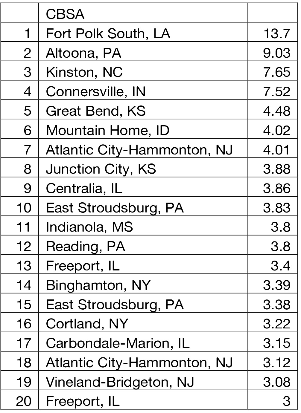
In Table 4 we show the highest 20 CBSA property tax rates as a percentage of value, based on mid-year estimated home values. Given that some jurisdictions do not re-assess property values as often as others, it is possible that some of the high figures will be dropping over time and lag the change in true values.
Table 4: Property Taxes as a Percentage of Estimated Home Values Mid 2017
Local governments with high property taxes likely depress home values just as high land rents depress the value of manufactured housing. The reverse should also hold where very low property taxes, and other expenses like utilities, likely help to inflate home values. This may help explain the high home prices in Honolulu relative to incomes.
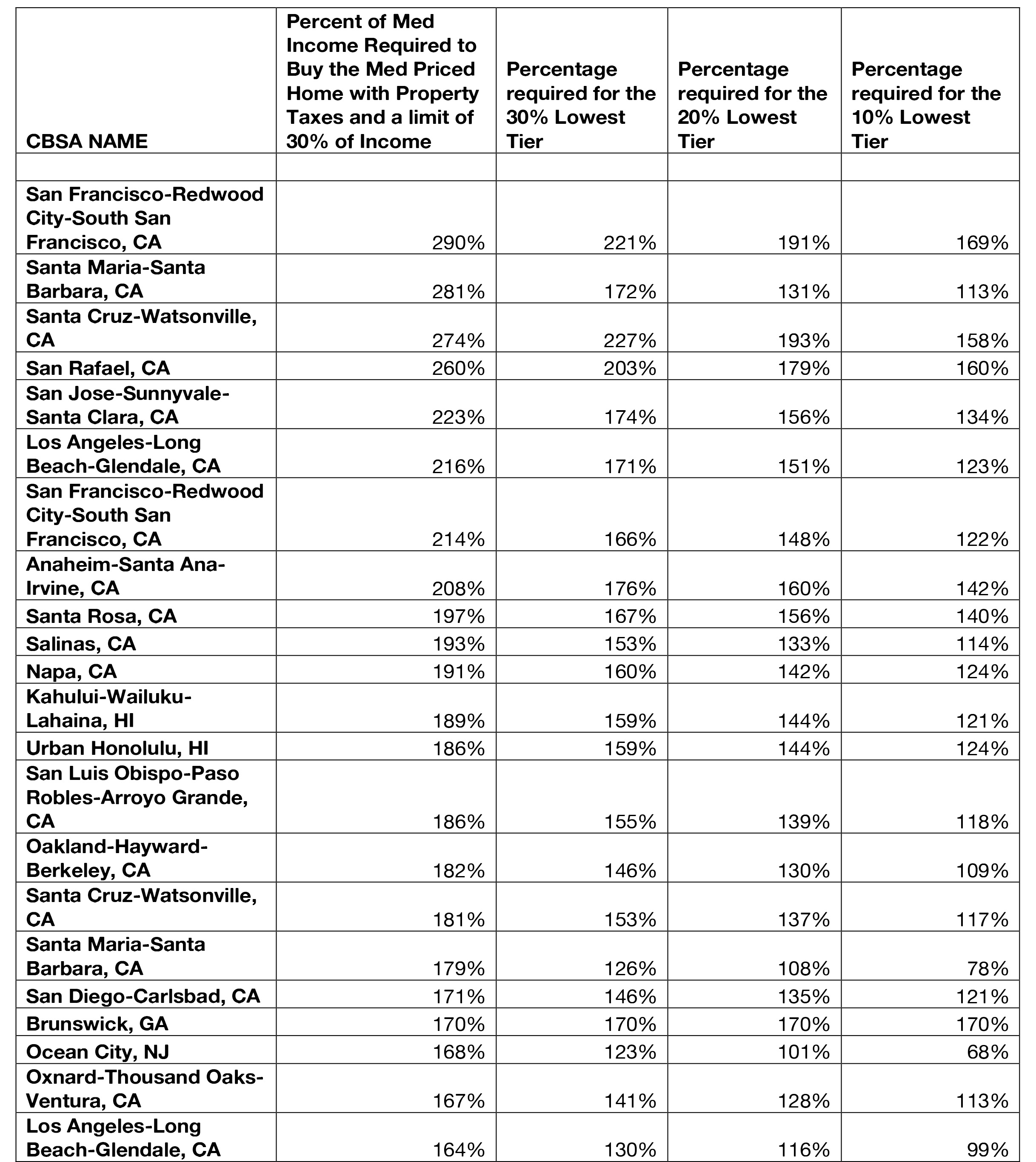
In Table 5 we show the combined results of property taxes and home prices, financed with an 80% loan to value mortgage, and this time using 30% of household income. The CBSA’s above in Table 4 all move up significantly on the unaffordable list but many do not enter the top 20 where price still dominates. Honolulu and Kahalui, both from Hawaii, move down the list while others from New Jersey, New York, Illinois, Pennsylvania and Tennessee move up the list. We also notice that some cities like Ocean City, NJ, while less affordable using median prices and income, are much more affordable at the 30% bottom tier level. This suggests a significant drop off from the median price to the 30% tier and also could suggest more impact on prices from the high property tax rates for the lowest price tiers of the market. More analysis will be necessary to examine the full impact of property taxes on prices.
Table 5: Combined Property Taxes and Home Prices
Conclusions
The notion of a perpetual housing crisis is fully consistent with the normal attributes of a capitalist economy, where some participants do better than others do, and where the political process can be used to inhibit supply in highly sought after locations. The lack of naturally occurring affordable housing in some high-supply-barrier markets can be mitigated, by allowing higher density housing, as we have witnessed more in markets like Chicago than in markets like San Diego. Still the problem will not go away any time soon. What we propose here is a more realistic way to approach the measurement of housing affordability in the owner market for entry-level housing.
Housing affordability measurements based on only median home prices and median household incomes are probably antiquated. Today, with richer data sets we can utilize more of the relevant information including segmenting the market into price tiers and considering actual property tax rates. A further refinement would consider the localized average loan to value ratio and this would help explain why Miami, FL or Sun City, NV are actually more affordable as the lower loan-to-value ratio typically used would be a way to incorporate the effect of wealth into the affordability calculation. Our results and proposed methodology are an alternative and we hope improved way to look at entry-level housing affordability.
References
CNBC.com published this report at 12:16 PM ET Wed, 13 Jan 2016, Interview of the CEO of Redfinm Glen Kelman.
Emmons, Gary, “No Place like Home: America’s Housing Crisis and Its Impact on Business” Harvard Business Review, March 20, 2000.
Lowry, Ira, Ira Lowry, “Rental Housing in the 1970’s: Searching for the Crisis” January, 1982, 74 page report, N-1833-HUD.
Weicher, John; Kevin Vallani and Elizabeth Roestacher, editors of Rental Housing: Is there a crisis? The Urban Institute Press, Wash. D.C. 1981.
Appendix 1: Related References on Regulatory Constraints on Land Use and Housing Prices
Aura, Saku and T. Davidoff. 2008. Supply Constraints and Housing Prices. Economics Letters 99(2): 275–277.
Davidoff, T. 2013. Supply Elasticity and the Housing Cycle of the 2000s. Real Estate Economics 41(4): 793–813.
Fischel, W. 1985. The Economics of Zoning Laws: A Property Rights Approach to American Land Use Controls. Baltimore, MD: Johns Hopkins University Press.
Foster, D.D. and A. Summers. 2005. Current State Legislative and Judicial Profiles on Land-use Regulations in the U.S. Working Paper, Zell/Lurie Real Estate Center, Wharton School, University of Pennsylvania.
Glaeser, E. and J. Gyourko. 2003. The Impact of Building Restrictions on Housing Affordability. Federal Reserve Bank of New York Economic Policy Review 9(2): 21-39.
Glaeser, E., J. Gyourko and R. Saks. 2005a. Why Is Manhattan So Expensive? Regulation and Rise in Housing Prices. Journal of Law and Economics 48(2): 331-370.
Glaeser, E., J. Gyourko and R. Saks. 2005b. Why Have Housing Prices Gone Up? American Economic Review 95(2): 329-333.
Glaeser, E., J. Schuetz and B. Ward. 2006. Regulation and the Rise of Housing Prices in Greater Boston. Cambridge, MA: Rappaport Institute for Greater Boston, Harvard University and Boston, MA: Pioneer Institute for Public Policy Research.
Glickfeld, M. and N. Levine. 1992. Regional Growth and Local Reaction: The Enactment and Effects of Local Growth Control and Management Measures in California. Cambridge, MA: Lincoln Institute of Land Policy.
Gyourko, J. and A.A. Summers. 2006a. The Wharton Survey on Land Use Regulation: Documentation and Analysis of Survey Responses. Working Paper, Zell/Lurie Real Estate Center, Wharton School, University of Pennsylvania.
Gyourko, J. and A.A. Summers. 2006b. Residential Land Use Regulation in the Philadelphia MSA. Working Paper, Zell/Lurie Real Estate Center, Wharton School, University of Pennsylvania.
Hilber, C.A.L. and F. Robert-Nicoud. 2013. On the Origins of Land Use Regulations: Theory and Evidence from U.S. Metro Areas. Journal of Urban Economics 75: 29–43.
Huang, H. and Y. Tang. 2012. Residential Land Use Regulation and the U.S. Housing Price Cycle between 2000 and 2009. Journal of Urban Economics 71: 93–99.
Hsieh, C.T. and E. Moretti 2015, “Housing Constraints and Spatial Miss-allocation” NBER Working Paper No. 21154. Updated May 18, 2017.
Ihlanfeldt, K. 2007. The Effect of Land Use Regulation on Housing and Land Prices. Journal of Urban Economics 61: 420-435.
Ihlanfeldt, K. and G. Burge. 2006a. The Effects of Impact Fees on Multifamily Housing Construction. Journal of Regional Science 46(1): 5-23.
Ihlanfeldt, K. and G. Burge. 2006b. Impact Fees and Single-family Home Construction. Journal of Urban Economics 60(2): 284-306.
Katz, L. and K.T. Rosen. 1987. The Interjurisdictional Effects of Growth Controls on Housing Prices. Journal of Law and Economics 30(1): 149-160.
Kolko, J. 2008. Did God Make San Francisco Expensive? Topography, Regulation, and Housing Prices. Working Paper, Public Policy Institute of California.
Levine, N. 1996. The Effects of Local Growth Controls on Regional Housing Production and Population Redistribution in California. Urban Studies 36(12): 2047-2068.
Malpezzi, S. 1996. Housing Prices, Externalities, and Regulation in U.S. Metropolitan Areas. Journal of Housing Research 7(2): 209-241.
Mayer, C. and S. Raphael. 2004. Land Use Regulation and New Construction. Regional Science and Urban Economics 30(6): 639-662.
Noam, E. 1983. The Interaction of Building Codes and Housing Prices. Journal of the American Real Estate and Urban Economics Association 10(4): 394-403.
Paciorek, A. 2013. Supply Constraints and Housing Market Dynamics. Journal of Urban Economics 77: 11-26.
Pendall, R., R. Puentes, and J. Martin. 2006. From Traditional to Reformed: a Review of the Land Use Regulations in the Nation’s 50 Largest Metropolitan Areas. Washington, DC: The Brookings Institution, Metropolitan Policy Program.
Pollakowski, H.O. and S.M. Wachter. 2000. The Effects of Land-Use Constraints on Housing Prices. Land Economics 66(3): 315-324.
Quigley, J.M. 2007. Regulation and Property Values in the United States: the High Cost of Monopoly. In Land Policies and Their Outcomes. G. Imgram and Y.H. Hong, eds. Cambridge, MA: Lincoln Institute of Land Policy. 46-66.
Quigley, J.M. and L. Rosenthal. 2005. The Effects of Land Regulation on the Price of Housing What Do We Know? What Can We Learn? Cityscape 8(1): 69-137.
Quigley, J.M. and S. Raphael. 2004. Is Housing Affordable? Why Isn’t It More Affordable? Journal of Economic Perspectives 18(1): 129-152.
Quigley, J.M. and S. Raphael. 2005. Regulation and the High Cost of Housing in California. American Economic Review 94(2): 323-328.
Rose, L.A. 1989. Topographical Constraints and Urban Land Supply Indexes. Journal of Urban Economics 26(3): 335-347.
Rose, L.A., and S.J. La Croix. 1989. Urban Land Price: The Extraordinary Case of Honolulu, Hawaii. Urban Studies 26(3): 301-314.
Saiz, A. 2010. The Geographic Determinants of Housing Supply. The Quarterly Journal of Economics 125(3): 1253-1296.
Sraer, D., T. Chaney, and D. Thesmar. 2012. The Collateral Channel: How Real Estate Shocks Affect Corporate Investment. The American Economic Review 102(6): 2381-2409.
Wallace, N.E. 1998. The Market Effects of Zoning Undeveloped Land Parcels: Does Zoning Follow the Market? Journal of Urban Economics 23(3): 307-326.
Appendix 2: Methods Used by NAR, HUD and CAR
- NAR National Association of REALTORS®
https://www.nar.realtor/research-and-statistics/housing-statistics/housing-affordability-index
- Definition of methods and assumptions (INDEX vs. DISTRIBUTION CURVE/SCORE)
- The Housing Affordability Index measures whether or not a typical family earns enough income to qualify for a mortgage loan on a typical home at the national and regional levels based on the most recent price and income data.
- A typical home is defined as the national median-priced, existing single-family home as calculated by NAR.
- The typical family is defined as one earning the median family income as reported by the U.S. Bureau of the Census.
- The prevailing mortgage interest rate is the effective rate on loans closed on existing homes from the Federal Housing Finance Board.
- These components are used to determine if the median income family can qualify for a mortgage on a typical home.
- FOR MORE INFO ON METHODOLOY
- REALTORS® Affordability Distribution Curve and Score
- The REALTORS® Affordability Distribution Curve and Score measures housing affordability at different income percentiles for all active inventory on the market. For each state, REALTORS® Affordability Distribution Curve shows how many houses are affordable to households ranked by income while REALTORS® Affordability Distribution Score is the measure which is intended to represent affordability for all different income percentiles in a single measure.
- The REALTORS® Affordability Distribution Score is different in two major ways from the existing Housing Affordability Index (HAI):
- It considers affordability for all income percentiles, not just the median income, and
- It looks at affordability of active inventory or homes currently available for sale instead of homes that have already sold.
- nar.realtor/research-and-statistics/housing-statistics/realtors-affordability-distribution-curve-and-score
- Monthly quarterly or annual housing affordability index by metro or market
-
- Definition of methods and assumptions
- The Location Affordability Portal is the product of a collaboration between HUD and the Department of Transportation (DOT) under the federal Partnership for Sustainable Communities. The Partnership, which includes the Department of Housing and Urban Development, the Department of Transportation, and the Environmental Protection Agency, works to coordinate federal housing, transportation, water, and other infrastructure investments to make neighborhoods more prosperous, allow people to live closer to jobs, save households time and money, and reduce pollution. One objective of this collaboration is to increase public access to data on housing, transportation, and land use. EPA’s Smart Location Database and EJSCREEN tools and HUD’s forthcoming AFFH Data Tool are other resources developed for this purpose.
- The prevailing standard of affordability in the United States is paying 30 percent or less of your family’s income on housing, which fails to account for for transportation costs. One reason is that transportation costs are a much bigger factor now than in the past. According to the Bureau of Labor Statistics, in the 1930’s American households spent just 8 percent of their income on transportation. Since then, as millions of families have migrated from center cities to surrounding suburbs and exurbs and come to rely more heavily on cars, that percentage has steadily increased, peaking at 19.1 percent in 2003. Today, households spend on average about 17 percent of their annual income on transportation, second only to housing costs in terms of budget impact. And for many-working class and rural households, transportation costs actually exceed housing costs.
- Before this Portal, though, there was no accurate, standardized data source on household transportation expenses, which limited the ability of homebuyers and renters to fully account for the cost of living in a particular city or neighborhood. This site seeks to fill that gap.
- Planners, policymakers, and developers also stand to benefit from access to this data when making decisions about land use, housing, transportation, and economic development. HUD and DOT have engaged experts and key stakeholders from the fields of urban and transportation planning, affordable housing, and economic development and produced extensive reviews of the data and modeling techniques used in the tools that have been made available on this site for the first time.
- Monthly quarterly or annual housing affordability index by metro or market
- The website looks like it has the ability to pull data by specific market but my internet is having issues with pulling up the graphs Affordability by metro is listed on: https://www.nar.realtor/sites/default/files/reports/2017/embargoes/2017-q1-metro-home-prices/metro-affordability-2016-existing-single-family-2017-05-15.pdf
- HUD Housing and Urban Development
https://egis-hud.opendata.arcgis.com/datasets/c1c32742599a42c9a45c95be50ed2ab6_0
- The website looks like it has the ability to pull data by specific market but my internet is having issues with pulling up the graphs Affordability by metro is listed on: https://www.nar.realtor/sites/default/files/reports/2017/embargoes/2017-q1-metro-home-prices/metro-affordability-2016-existing-single-family-2017-05-15.pdf
- California Association of Realtors®
http://www.car.org/marketdata/data/haitraditional/?highlight=affordability
- Definition of methods and assumptions
- C.A.R.’s Traditional Housing Affordability Index (HAI) measures the percentage of households that can afford to purchase the median priced home in the state and regions of California based on traditional assumptions. C.A.R. also reports its traditional and first-time buyer indexes for regions and select counties within the state. The HAI is the most fundamental measure of housing well-being for buyers in the state.
- THE ASSUMPTIONS AND METHODOLOGY USED TO CALCULATE C.A.R.’S TRADITIONAL HOUSING AFFORDABILITY INDEX (HAI)
- Step 1. MEDIAN PRICE: C.A.R.’s housing affordability index is based on the median price of existing single-family homes sold from C.A.R.’s monthly existing home sales survey. Starting in 1987, this survey is based on reports of closed escrow sales from 80 Boards or more of REALTORS® and multiple listing services around the state. Prior to 1987, the survey was based on reports from 45 Boards.
- Step 2. DOWN PAYMENT: It is assumed that a household can make a 20 percent down payment on the median-priced home. Therefore, the loan amount needed to purchase a home would be 80 percent of the median home sales price.
- Step 3. INTEREST RATE: Using the national average effective mortgage interest rate on all fixed and adjustable rate mortgages. This is represented by the effective composite rate for previously occupied homes, which is reported monthly by the Federal Housing Finance Board.
- Step 4.The monthly payment for PRINCIPAL, INTEREST, TAXES AND INSURANCE (PITI) is computed as the sum of three parts:
- Monthly mortgage payment, based on the terms of the mortgage in Steps 2 & 3.
- Monthly PROPERTY TAXES are assumed to be 1 percent of the median home sales price divided by 12.
- Monthly INSURANCE PAYMENTS on the house are assumed to be 0.38 percent of the median home sales price divided by 12.
- The results of these three calculations are added together to find the PITI or total monthly payment for a household that buys the median priced home.
- Step 5. It is then assumed that the monthly PITI can be no more than 30 percent of a household’s income. Thus, the monthly housing payment is divided by .3 to come up with the MINIMUM INCOME NEEDED TO QUALIFY FOR A LOAN on the median-priced home.
- Step 6. Starting in 1988, data for the distribution of households by various income ranges was obtained from Claritas. INCOME DISTRIBUTION figures were developed based on the projected percent change in the annual median household income. Prior to 1988, household income utilized in the housing affordability index was based on projections by C.A.R. using the 1980 census data as a base.
- Step 7. The minimum income amount calculated in Step 5 is multiplied by 12 to determine the minimum annual income needed to qualify. This amount is compared to the income distribution of households. The percent of the households with incomes greater than or equal to the minimum income becomes the HOUSING AFFORDABILITY INDEX (HAI).
- NOTE: The quarterly HAI series begins in 2006, prior to that the series was monthly. The quarterly HAI for a given geographic area in a particular quarter is based upon the quarterly median price for that area as well as the quarterly income distribution for that area.
- Definition of methods and assumptions
-
- The Housing Affordability Index measures whether or not a typical family earns enough income to qualify for a mortgage loan on a typical home at the national and regional levels based on the most recent price and income data.
[1] Published September 12th, 2017 in an economic outlook blog titled “Ten years from the last crash, is another global housing bubble underway?” by CBRE.
[2] See Ira Lowry, “Rental Housing in the 1970’s: Searching for the Crisis” January, 1982, 74 page report, N-1833-HUD, for the department of Housing and Urban Development. Also see John Weicher, Kevin Vallani and Elizabeth Roestacher, editors of Rental Housing: Is there a crisis? The Urban Institute Press, Wash. D.C. 1981.
[3] See Gary Emmons, No Place like Home: America’s Housing Crisis and Its Impact on Business” Harvard Business Review, March 20, 2000.
[4] CNBC.com published this report at 12:16 PM ET Wed, 13 Jan 2016
[5] For example, in high priced markets like La Jolla, CA. we observe LTVs averaging 55% and even lower on the larger homes. In National City, CA, where home prices are now about $375,000 we observe average LTVs of 93%.
[6] Source: National Association of REALTORS® but available at https://fred.stlouisfed.org/series/COMPHAI
[7] See the references for work by Ed Glaeser, Joe Gyourko, Anita Summers and Albert Saiz among others demonstrating how regulations and restrictions on supply are the primary determinant of land prices and housing costs, which in turn, make housing less or more affordable.
Appendix 2 includes a review of methodologies used by NAR, HUD and the California Association of REALTORS®.